The ability to perform calculation of a gas producing system, including the reservoir and the piping system, requires knowledge of many gas properties at various pressures and temperatures. If the natural gas is in contact with liquids, such as condensate or water, the effect of the liquids on gas properties must be evaluated.
- Ideal Gases
- Early Gas Laws
- The Ideal Gas Law
- Ideal Gas Mixtures
- Apparent Molecular Weight
- Real Gases
- Real Gas Mixtures
- Gas Formation Volume Factor
- Correction for Nonhydrocarbon Impurities
- Other Equations of State
- Benedict-Webb-RubIn Equation (BWR)
- Rediich-Kwong Equation (RK)
- Gas Isothermal Compressibility
- Ideal Gas Compressibility
- Real Gas Compressibility
- Gas Viscosity
- Gas-Water Systems
- Solubility of Natural Gas in Water
- Solubility of Water in Natural Gas
- Solubility of Water in Natural Gas
- Gas Hydrates
- Gas-Condensate Systems
- Phase Behavior
- Types of Gas Reservoirs
- Flash or Equilibrium Separation Calculations
- Determination of Equillibrium Ratios
- K-Values from Equations of State
- Adjustment of Properties for Condensate Mixtures
This article presents the best and most widely used methods to perform the necessary calculations. Some of the information presented in this article will be used only in reservoir calculations and some will be used only in the piping system design article; therefore, this article will be referred to frequently in the subsequent articles.
Numerous example problems are worked and graphs are presented for empirical correlations. Application of some of the methods requires a computer, and FORTRAN subroutines are included in the appendix if available.
Ideal Gases
The understanding of the behavior of gases with re =spect to pressure and temperature changes is made clearer by first considering the behavior of gases at conditions near standard conditions of pressure and temperature; that is:
At these conditions the gas is said to behave ideally, and most of the early work with gases was conducted at conditions approaching these conditions.
An ideal gas is defined as one in which:
- The volume occupied by the molecules is small compared to the total gas volume;
- All molecular collisions are elastic;
- And there are no attractive or repulsive forces among the molecules.
The basis for describing ideal gas behavior comes from the combination of some of the so-called gas laws proposed by early experimenters.
Early Gas Laws
Boyle’s Law. Boyle observed experimentally that the volume of an ideal gas is inversely proportional to the pressure for a given weight or mass of gas when temperature is constant. This may be expressed as:
Charles’ Law. While working with gases at low pressures, Charles observed that the volume occupied by a fixed mass of gas is directly proportional to its absolute temperature, or:
Avogadro’s Law. Avogadro’s Law states that under the same conditions of temperature and pressure, equal volumes of all ideal gases contain the same number of molecules. This is equivalent to the statement that at a given temperature and pressure one molecular weight of any ideal gas occupies the same volume as one molecular weight of another ideal gas. It has been shown that there are 2,73×1026 molecules/lb-mole of ideal gas and that one molecular weight in pounds of any ideal gas at 60 °F and 14,7 psia occupies a volume of 379,4 cu ft. One mole of a material is the quantity of that material whose mass, in the system of units selected, is numerically equal to the molecular weight. This means that one mole of any ideal gas, that is, 2,73×1026 molecules of any gas, will occupy the same volume at a given pressure and temperature.
The Ideal Gas Law
The three gas laws described previously can be combined to express a relationship among pressure, volume, and temperature, called the ideal gas law.
In order to combine Charles’ Law and Boyle’s Law to describe the behavior of an ideal gas when both temperature and pressure are changed, assume a given mass of gas whose volume is V1 at pressure p1 and temperature T1, and imagine the following process through which the gas reaches volume V2, at pressure p2, and temperature T2:
In the first step the pressure is changed from a value of p1 to a value of p2 while temperature is held constant. This causes the volume to change from V1 to V. In Step 2, the pressure is maintained constant at a value of p2 and the temperature is changed from a value of T1 to a value of T2.
The change in volume of the gas during the first step may be described through the use of Boyle’s Law since the quantity of gas and the temperature are held constant. Thus:
where:
- V – represents the volume at pressure p2 and temperature T1.
Charles’ Law applies to the change in the volume of gas during the second step since the pressure and the quantity of gas are maintained constant; therefore:
Elimination of volume, V, between Equations 1 and 2 gives:
or:
Thus for a given quantity of gas, pV/T = a constant. The constant is designated with the symbol R when the quantity of gas is equal to one molecular weight. That is:
where:
- VM – is the volume of one molecular weight of the gas at p and T.
In order to show that R is the same for any gas, Avogadro’s Law is invoked. In symbolic form, this law states:
where:
- VMA – represents the volume of one molecular weight of gas A and;
- VMB – represents the volume of one molecular weight of gas B;
- Both at pressure, p, and temperature, T.
This implies that:
and:
where:
- RA – represents the gas constant for gas A and;
- RB – represents the gas constant for gas B.
The combination of the above equations reveals that:
Thus, the constant R is the same for all ideal gases and is referred to as the universal gas constant. Therefore, the equation of state for one molecular weight of any ideal gas is:
For n moles of ideal gas this equation becomes:
where:
- V – is the total volume of n moles of gas at temperature, T, and pressure, p.
Since n is the mass of gas divided by the molecular weight, the equation can be written as:
or, since m/V is the gas density:
This expression is known by various names such as the ideal gas law, the general gas law, or the perfect gas law. This equation has limited practical value since no known gas behaves as an ideal gas; however, the equation does describe the behavior of most real gases at low pressure and gives a basis for developing equations of state which more adequately describe the behavior of real gases at elevated pressures.
The numerical value of the constant R depends on the units used to express temperature, pressure, and volume. As an example, suppose that pressure is expressed in psia, volume in cubic feet, temperature in degrees Rankin, and moles in pound moles. Avogadro’s Law states that lib-mole of any ideal gas occupies 379,4 cu ft at 60 °F and 14,7 psia. Therefore:
Table 1 gives numerical values of R for various systems of units.
Example 1:
Calculate the mass of methane gas contained at 1 000 psia and 68 °F in a cylinder with volume of 3,20 cu ft. Assume that methane is an ideal gas.
Solution:
Example 2:
Calculate the density of methane at standard conditions.
| Table 1. Values of Gas Constant R in Various Units | |
|---|---|
| Units | R |
| atm, cc/g-mole, °K | 82,06 |
| BTU/lb-mole, °R | 1,987 |
| psia, cu ft/lb-mole, °R | 10,73 |
| lb/sq ft abs, cu ft/lb-mole, °R | 1 544 |
| atm, cu ft/lb-mole, °R | 0,730 |
| mm Hg, liters/g-mole, °K | 62,37 |
| in. Hg, cu ft/lb-mole, °R | 21,85 |
| cal/g-mole, °K | 1,987 |
| kPa, m3/kg-mole, °K | 8,314 |
| J/kg-mole, °K | 8 314 |
Ideal Gas Mixtures
The previous treatment of the behavior of gases applies only to single component gases. As the gas engineer rarely works with pure gases, the behavior of a multicomponent mixture of gases must be treated. This requires the introduction of two additional ideal gas laws.
Dalton’s Law. Dalton’s Law states that each gas in a mixture of gases exerts a pressure equal to that which it would exert if it occupied the same volume as the total mixture. This pressure is called the partial pressure. The total pressure is the sum of the partial pressures. This law is valid only when the mixture and each component of the mixture obey the ideal gas law. It is sometimes called the Law of Additive Pressures.
The partial pressure exerted by each component of the gas mixture can be calculated using the ideal gas law. Consider a mixture containing nA moles of component A, nB moles of component B and nC moles of component C. The partial pressure exerted by each component of the gas mixture may be determined with the ideal gas equation:
According to Dalton’s Law, the total pressure is the sum of the partial pressures:
It follows that the ratio of the partial pressure of component j, pj, to the total pressure of the mixture p is:
where:
- yj – is defined as the mole fraction of the jth component in the gas mixture.
Therefore, the partial pressure of a component of a gas mixture is the product of its mole fraction times the total pressure.
Amagat’s Law. Amagat’s Law states that the total volume of a gaseous mixture is the sum of the volumes that each component would occupy at the given pressure and temperature. The volumes occupied by the individual components are known as partial volumes. This law is correct only if the mixture and each of the components obey the ideal gas law.
The partial volume occupied by each component of a gas mixture consisting of nA moles of component A, nB moles of component B, and so on, can be calculated using the ideal gas law:
Thus, according to Amagat, the total volume is:
It follows that the ratio of the partial volume of component j to the total volume of the mixture is:
This implies that for an ideal gas the volume fraction is equal to the mole fraction.
Apparent Molecular Weight
Since a gas mixture is composed of molecules of various sizes, it is not strictly correct to say that a gas mixture has a molecular weight. However, a gas mixture behaves as if it were a pure gas with a definite molecular weight. This molecular weight is known as an apparent molecular weight and is defined as:
Example 3:
Dry air is a gas mixture consisting essentially of nitrogen, oxygen, and small amounts of other gases. Compute the apparent molecular weight of air given its approximate composition. The molecular weight of each component may be found in Table 2.
| Component | Mole fraction, yj |
|---|---|
| Nitrogen | 0,78 |
| Oxygen | 0,21 |
| Argon | 0,01 |
| 1,00 |
Solution:
A value of 29,0 is usually considered sufficiently accurate for engineering calculations.
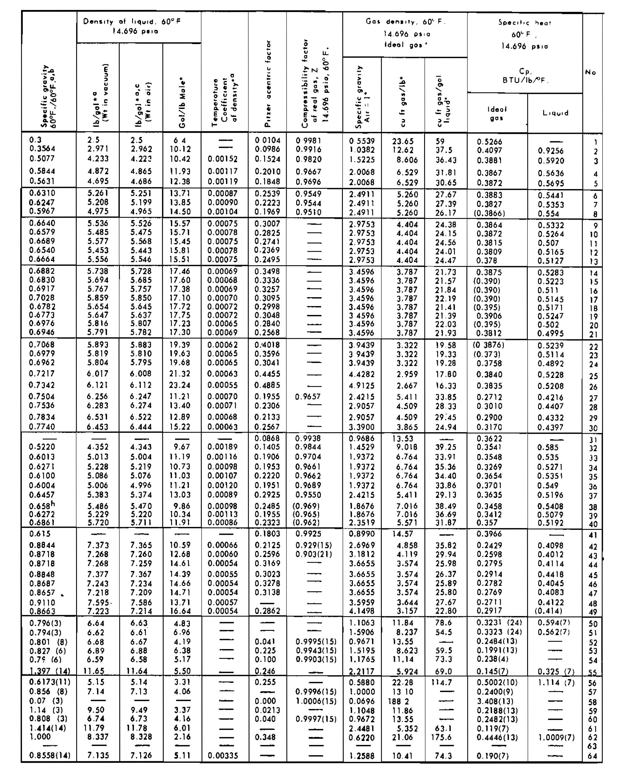
The specific gravity of a gas is defined as the ratio of the density of the gas to the density of dry air taken at standard conditions of temperature and pressure. Symbolically:
Assuming that the behavior of both the gas and air may be represented by the ideal gas law, specific gravity may be given as:
where:
- Mair – is the apparent molecular weight of air.
If the gas is a mixture, this equation becomes:
where:
- Ma – is the apparent molecular weight of the gas mixture.
Example 4:
Calculate the gravity of a natural gas of the following composition.
| Component | Mole fraction, yj |
|---|---|
| Methane | 0,85 |
| Ethane | 0,09 |
| Propane | 0,04 |
| n-butane | 0,02 |
| 1,00 |
Solution:
| Component | Mole fraction, yj | Molecular weight, Mj | yjMj |
|---|---|---|---|
| C1 | 0,85 | 16,0 | 13,60 |
| C2 | 0,09 | 30,1 | 2,71 |
| C3 | 0,04 | 44,1 | 1,76 |
| n-C4 | 0,02 | 58,1 | 1,16 |
| 1,00 | 19,23 = Ma |
Real Gases
Several assumptions were made in formulating the equation of state for ideal gases. Since these assumptions are not correct for gases at pressures and temperatures that deviate from ideal or standard conditions, corrections must be made to account for the deviation from ideal behavior. The most widely used correction method in the petroleum industry is the gas compressibility factor, more commonly called the Z-factor. It is defined as the ratio of the actual volume occupied by a mass of gas at some pressure and temperature to the volume the gas would occupy if it behaved ideally. That is:
The equation of state is:
Therefore, the equation of state for any gas becomes:
where:
- For an ideal gas, Z = 1.
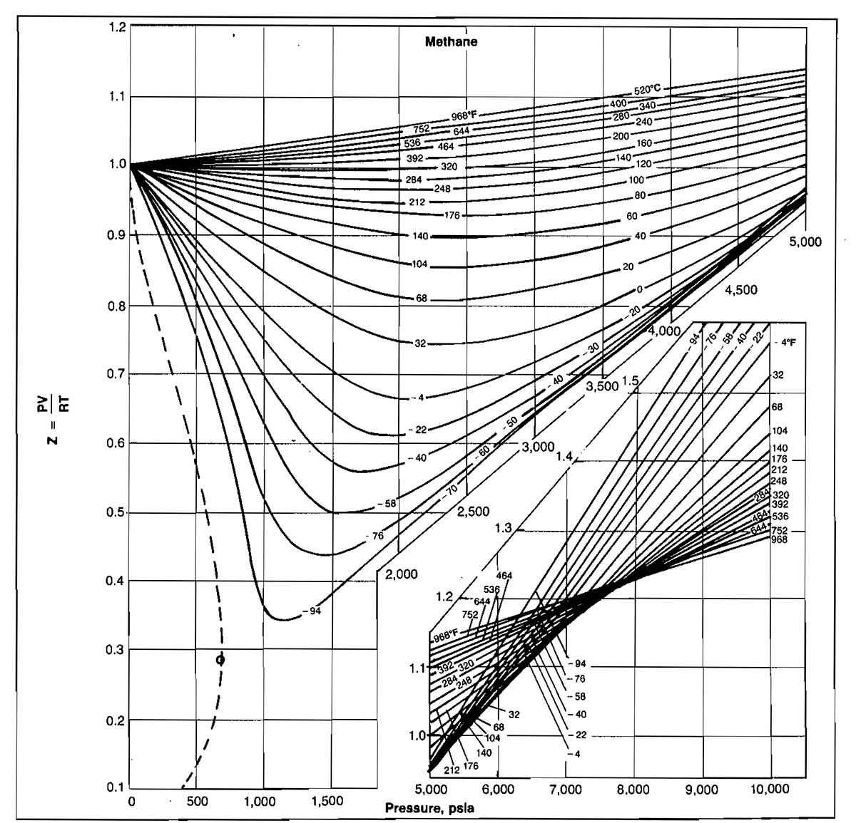
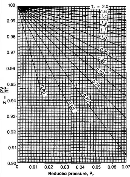
The compressibility factor varies with changes in gas composition, temperature, and pressure. It must be detennined experimentally. The results of experimental determinations of compressibility factors are normally given graphically and usually take the form shown in Picture 1.
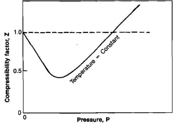
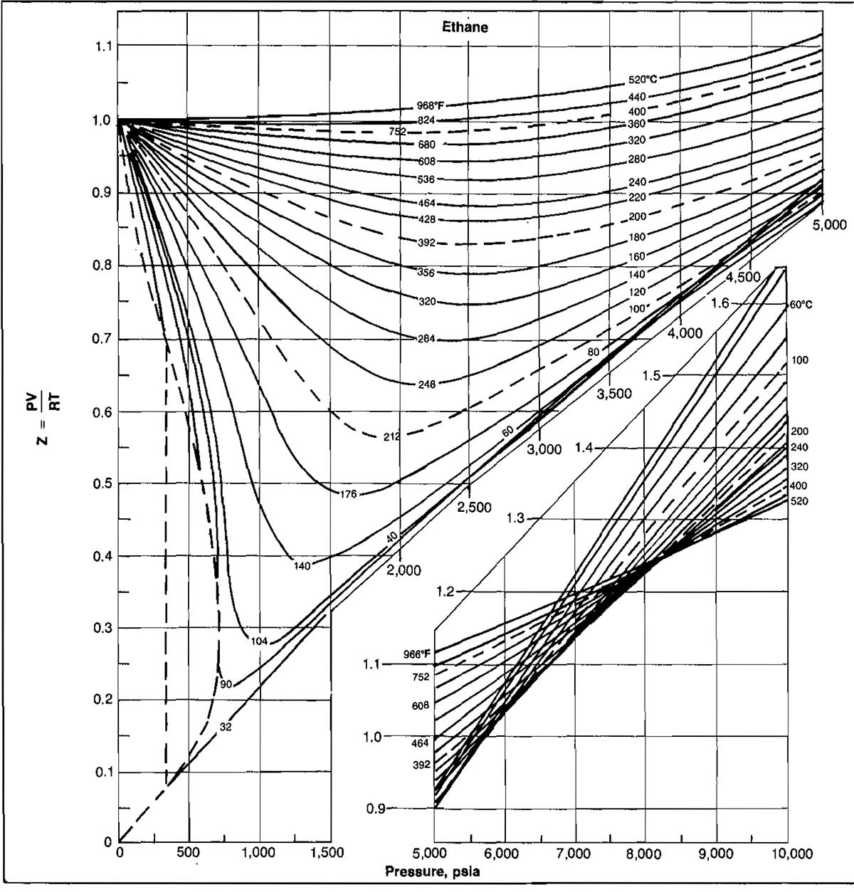
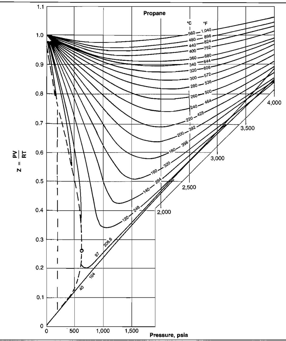
The shape of the curve is consistent with present knowledge of the behavior of gases; at very low pressure the molecules are relatively far apart and the conditions of ideal gas behavior are more likely to be met. At low pressure the compressibility factor approaches a value of 1,0, which would indicate that ideal gas behavior does in fact occur. Compressibility factors for several hydrocarbon gases are given in Pictures 2, 3, and 4.
Example 5:
Calculate the mass of methane gas contained at 1 000 psia and 68 °F in a cylinder with volume of 3,20 cu ft.
Solution:
Z = 0,89 (from Picture 2).
If ideal behavior had been assumed, the mass calculated would have been m = 10,2 (.89) = 9,08 lmb.
Real Gas Mixtures
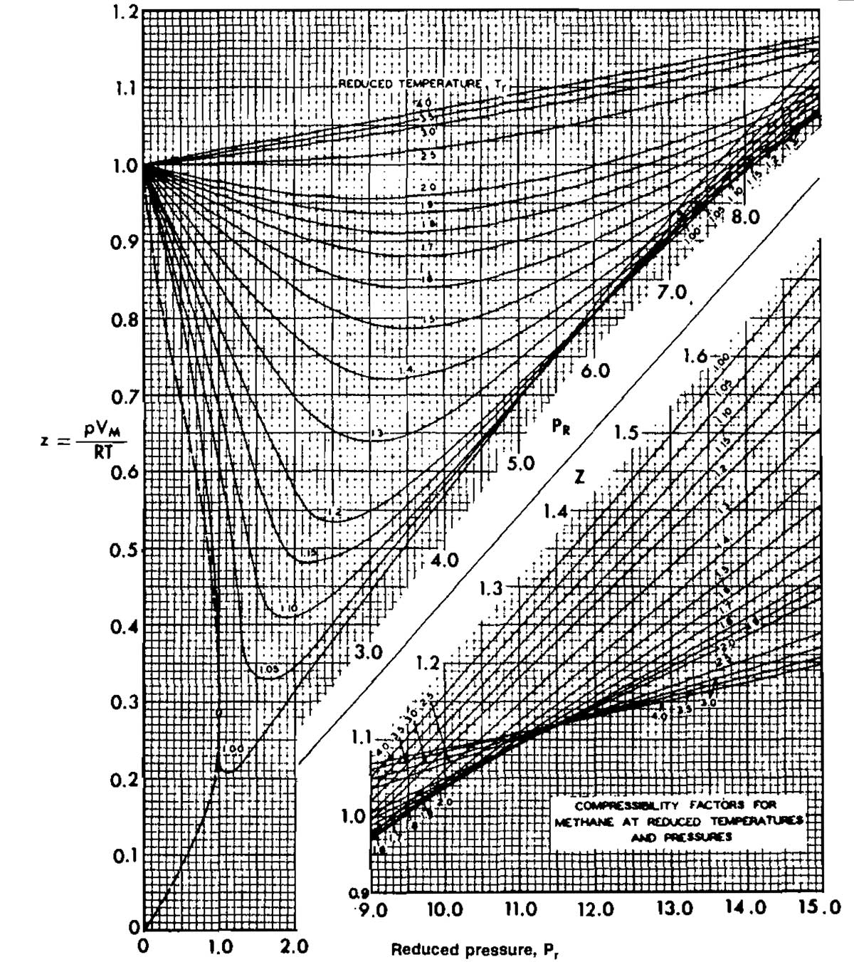
Compressibility factor charts are available for most of the single component light hydrocarbon gases, but in practice a single component gas is rarely encountered. In order to get Z-factors for natural gas mixtures, the law of corresponding states is used. This law states that the ratio of the value of any intensive property to the value of that property at the critical state is related to the ratios of the prevailing absolute temperature and pressure to the critical temperature and pressure by the same function for all similar substances. This means that all pure gases have the same Z-factor at the same values of reduced pressure and temperature, where the reduced values are defined as:
where:
- Tc and pc are the critical temperature and pressure for the gas, respectively. The values must be in absolute units.
Example 6:
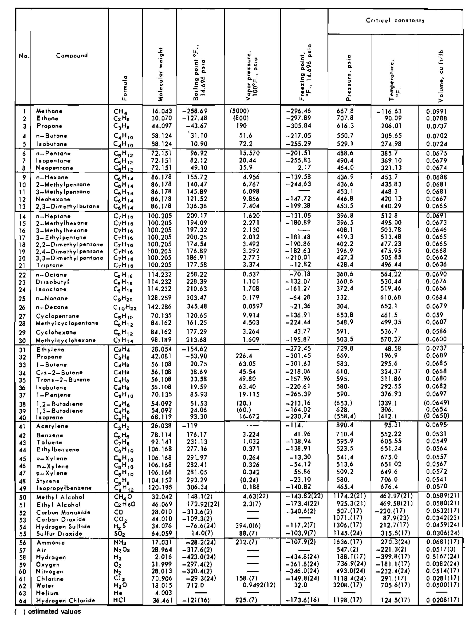
Calculate the density of ethane at 900 psia and 110 °F. The critical properties, from Table 2, are:
- Tc = 550 °R;
- pc = 708 psia;
- M = 30,1 lbm/lb-mole.
Solution:
From Picture 5, Z ≈ 0,34.
Assuming ideal behavior, the value calculated would be ρ = 13,03 (.34) = 4,43 lbm/ft3.
It has been shown that the Law of Corresponding States works better for gases of similar molecular characteristics. This is fortunate since most of the gases that the petroleum engineer deals with are composed of molecules of the same class of organic compounds known as paraffin hydrocarbons. The law of corresponding states has been extended to cover mixtures of gases that are closely related chemically. Since it is somewhat difficult to obtain the critical point for multicomponent mixtures, the quantities of pseudocritical temperature and pseudocritical pressure have been conceived.
These quantities are defined as:
These pseudocritical quantities are used for mixtures of gases in exactly the same manner as the actual critical temperatures and critical pressures are used for pure gases. It must be understood, however, that these pseudocritical properties were devised simply for use in correlating compressibility factors and in no way relate to the actual critical properties of the gas mixture.
Example 7:
Calculate the pseudocritical temperature and pseudocritical pressure of the following natural gas mixture. Use the critical constants given in Table 2.
Solution
| Component | Mole fraction yj | Critical temperature, °R. Tcj | yjTcj | Critical pressure, psia pcj | yjpcj |
|---|---|---|---|---|---|
| C1 | 0,85 | 343,1 | 291,6 | 667,8 | 567,6 |
| C2 | 0,09 | 549,8 | 49,5 | 707,8 | 63,7 |
| C3 | 0,04 | 865,7 | 26,6 | 616,3 | 24,7 |
| n-C4 | 0,02 | 765,3 | 15,3 | 550,7 | 11,0 |
| 1,00 | Tpc = 383,0 °R | ppc = 667,0 psla |
The compressibility factors for natural gases have been correlated using pseudocritical properties and are presented in Pictures 6, 7, and 8.


Compressibility factors are a function of composition as well as temperature and pressure. It has been pointed out that the components of most natural gases are hydrocarbons of the same family. and therefore a correlation of this type is possible.
Example 8:
Calculate the volume occupied by 1 lb-mole of the natural gas given in Example 7 at 120 °F and 1 500 psia.
Solution:
Z = 0,813 (from Pic. 2-6).
A computer subroutine for calculating Z-factor is given in the Appendix. This subroutine reproduces Picture 6.
In some cases the composition of a gas will be given in weight or mass percent rather than mole percent. In this event, the composition must be first converted to mole fraction or percent before the mixture properties can be calculated. The following example illustrates this conversion.
Example 9:
A gas mixture consists of 50 % C1, 30 % C2, and 20 % C3 by weight. Calculate the apparent molecular weight and specific gravity of this mixture.
Solution:
Assume 100 lbm of gas as a basis.
| Component | Mass, mj lbm | Mj lbm/lb-mole | nj, lb-mole | yj | yjMj |
|---|---|---|---|---|---|
| C1 | 50 | 16 | 3,13 | 0,68 | 10,9 |
| C2 | 30 | 30 | 1,00 | 0,22 | 6,6 |
| C3 | 20 | 44 | 0,45 | 0,10 | 4,4 |
| 100 | n = 4,58 | 1,00 | 21,9 |
If the volume fraction is given at conditions other than standard, the volume fraction must be converted to a mole fractions basis, taking into account the deviation from ideal behavior. The following example illustrates this procedure.
Example 10:
A gas has the following composition measured at 2 500 psia and 300 °F. Calculate the composition in mole fraction. The volume percents at these conditions are:
- C1 = 67 %;
- C2 = 30 %;
- C3 = 1 %;
- CO2 = 2 %.
Solution:
To convert from volume to moles, assume 100 ft3 as a basis. Then use:
| Component | Vj, ft3 | Tr | pr | Z | V/Z | nj | yj = nj/n |
|---|---|---|---|---|---|---|---|
| C1 | 67 | 2,20 | 3,72 | 0,963 | 69,6 | 21,30 | .595 |
| C2 | 30 | 1,40 | 3,53 | 0,708 | 42,5 | 13,00 | .363 |
| C3 | 1 | 1,14 | 4,06 | 0,585 | 1,8 | 0,55 | .015 |
| CO2 | 2 | 1,30 | 2,32 | 0,658 | 3,2 | 0,48 | .027 |
| 100 | n = 38,83 | 1,000 |
In most cases the composition of a natural gas will be known and the apparent molecular weight and critical properties can be calculated as previously described. Occasionally, however, only the gas gravity will be known. Also, it is very easy to measure the gas gravity in the field. If the composition is unknown, or if accuracy requirements do not justify the longer calculations, Picture 9 can be used to estimate the pseudocritical properties.
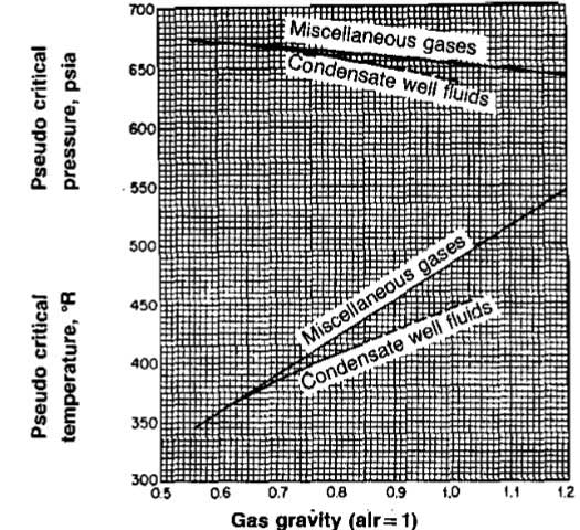
The properties can also be calculated using the following equations.
For condensate fluids:
Example 11:
Using the empirical correlation (Picture 9) for critical properties, calculate Tpc and ppc for the gas in Example 4. Compare these values with those obtained using the composition (Example 7).
Solution:
Gas Formation Volume Factor
In most operations involving gas production the flow rates and quantities produced are measured at standard conditions such as scf/day or scf, Reservoir engineering and pipeline flow calculations require the volumes at in situ conditions of pressure and temperature, and therefore a convenient conversion factor from standard conditions to in situ conditions is needed. This conversion factor is called the gas formation volume factor and is defined as the actual volume occupied by the gas at some pressure and temperature divided by the volume that the gas would occupy at standard conditions.
That is:
Using:
- Tsc = 520 °R;
- psc = 14,7 psia;
- Zsc = 1;
Gives:
It is sometimes convenient to express Bg in barrels of volume, or:
For the constant given above, pressure is in psia and temperature is in °R. For the SI system (p = kPa, T = °K):
Example 12:
Calculate the formation volume factor for a natural gas having a gravity of 0,7 at a temperature of 93 °C and an absolute pressure of 10 343 kPa.
Solution:
From Picture 6, Z = .88.
Correction for Nonhydrocarbon Impurities
Natural gases frequently contain materials other than hydrocarbons, such as nitrogen (N2), carbon dioxide (CO2), and hydrogen sulfide (H2S). The presence of these impurities affects the value obtained from the Z-factor chart.
A procedure for adjusting the critical properties of the gas was proposed by Wichert and Aziz in 1970. The adjusted critical properties are then used in calculating the reduced properties, and the Z-factor is then obtained from Picture 6.
The procedure for obtaining the Z-factor for sour gases is:
1 Determine ppc and Tpc for the gas using the gas composition or Picture 9 and;
2 Calculate the adjusted critical properties.
where:
- ∈ = 120(A0,9-A1,6)+15(B0,5-B4);
- B = mole fraction H2S;
- A = mole fraction CO2+B;
- ∈ = correction factor, °F.
3 Calculate the reduced properties using the corrected critical properties:
4 Find Z from Picture 6 or using the correlation given in the Appendix.
Example 13:
A gas containing 2,87 % CO2 and 23,27 % H2S has a critical pressure of 822 psia and a critical temperature of 465 °R. Find the gas compressibility factor, Z, for p = 1 000 psia, T = 100 °F.
Solution:
From Picture 6, Z = 0,78.
Other Equations of State
One of the limitations in the use of the compressibility equation to describe the behavior of gases is that the compressibility factor is not constant, and therefore mathematical manipulations cannot be made directly but must be accomplished through graphical or numerical techniques. Most of the other commonly used equations of state were devised so that the correction factors, which correct the ideal gas law for nonideality, may be assumed constant, thus permitting the equations to be used in mathematical calculations involving differentiation or integration.
Many equations of state have been proposed for describing gas behavior and many modifications and improvements have been made. Only two of the most commonly used equations will be described. These will be used later in the calculation of phase behavior.
Benedict-Webb-RubIn Equation (BWR)
An earlier equation presented by Beattie and Bridgeman was modified and resulted in an equation with eight empirical constants.
The parameters Bo, Ao, Co, a, b, c, α and γ are constants for pure compounds and are functions of composition for mixtures. The constants for pure compounds are given in Table 3.
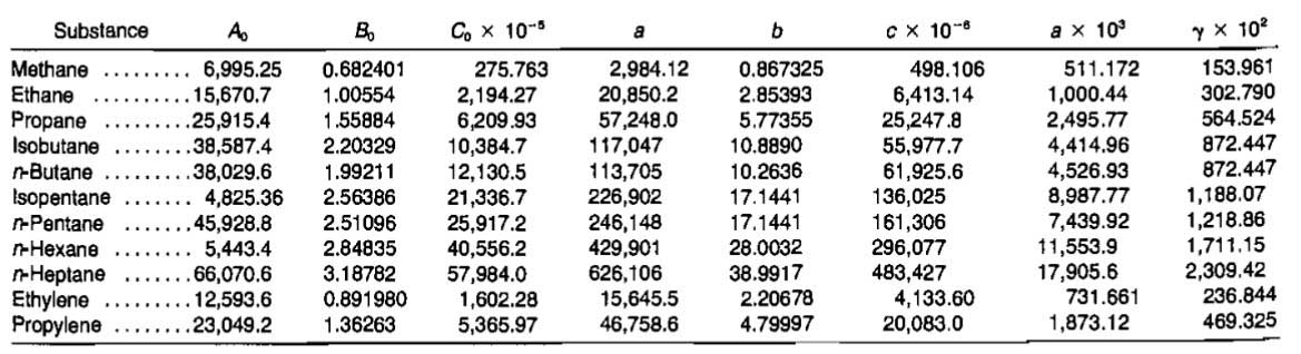
These constants may be combined for use with mixtures of gases according to the following mixture rules.
Rediich-Kwong Equation (RK)
The Redlich-Kwong Equation involves only two empirical constants as opposed to the eight required in the BWR equation. The original RK equation is:
where:
To simplify the calculations with the RK equation, especially for application to mixtures, other constants have been defined as:
where, for temperature in °R and pressure in psia:
- Ca = 0,42748;
- Cb = 0,08664.
The RK equation was further modified by Soave to improve its accuracy when applied to mixtures as follows:
where:
- α – is a function of temperature.
Using the following definitions, a gas compressibility factor can be calculated:
The constants A and B are calculated for mixtures by:
where:
- yi – is the mole fraction of the ith component of the mixture.
Evaluation of α involves calculation of the acentric factor, ω:
where:
- TB is the boiling point of the component at 14,7 psia in °R;
- Values of ω can also be obtained from Table 2.
Example 14:
Using the Soave modification to the RK equation, calculate the molar volume of the following gas mixture at p = 250 psia, T = 100 °F.
| Component | yj |
|---|---|
| C1 | 0,75 |
| C2 | 0,15 |
| C3 | 0,10 |
| 1,00 |
Solution:
| Component | yj | pcj | Tcj | ωj | Sj | αj |
|---|---|---|---|---|---|---|
| C1 | 0,75 | 667,8 | 343,4 | 0,0104 | 0,496 | 0,744 |
| C2 | 0,15 | 707,8 | 550,1 | 0,0986 | 0,633 | 0,989 |
| C3 | 0,10 | 616,3 | 666,1 | 0,1524 | 0,716 | 1,123 |
| Component | ||
|---|---|---|
| C1 | 8,597 | 0,38567 |
| C2 | 3,084 | 0,11658 |
| C3 | 2,843 | 0,10808 |
| 14,524 | 0,61033 |
Calculations for C1:
From Table 2, ω = 0,0104.
Gas Isothermal Compressibility
The isothermal compressibility of a gas is the measure of the change in volume per unit volume with pressure change at constant temperature. In equation form:
This should not be confused with the gas compressibility factor, Z. The compressibility is required in many reservoir gas flow equations and may be evaluated in the following manner.
Ideal Gas Compressibility
For an ideal gas:
and therefore:
Real Gas Compressibility
For a real gas:
and since Z = f(p), it must be included in the derivative:
Substituting these expressions into the equation defining compressibility gives:
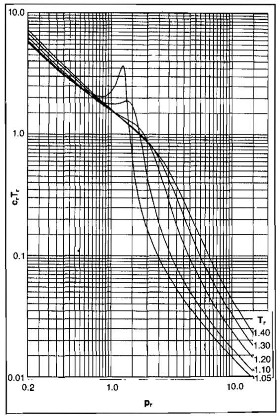
Evaluation of C for real gases requires determining how the Z-factor varies with pressure at the pressure and temperature of interest. Because most of the charts and equations predict Z as a function of reduced pressure and temperature, a reduced compressibility has been defined as Cr = C pc.
This can be expressed as a function of pr at a fixed value of Tr by:
Values of
can be obtained from the slope of a constant Tr curve from Picture 6 at the Z-factor of interest. Values of Cr Tr as a function of pr and Tr have been presented graphically by Mattar, et al. in Pictures 10 and 11.

The change of Z with p can also be calculated using an analytical expression by calculating the Z-factor at pressures slightly above and below the pressure of interest. That is:
Example 15:
Calculate the compressibility of a gas at a temperature of 40 °F and a pressure of 665 psia if Tc = 357 °R, pc = 674 psia.
Solution:
From Picture 11, Cr Tr = 1,62.
The problem can also be solved using the approximation for ∂Z/∂pr:
| p, psia | pr | Z |
|---|---|---|
| 615 | 0,912 | 0,880 |
| 665 | 0,986 | 0,870 |
| 715 | 1,060 | 0,861 |
Gas Viscosity
The viscosity of a fluid is a measure of the fluid’s ability to flow, or the ratio of the shearing force to the shearing rate. The viscosity is usually expressed in centipoises or poises, but can be converted to other units for unit compatibility.
Gas viscosity is difficult to measure experimentally and for engineering purposes can be determined accurately enough from empirical correlations. The most widely accepted correlation used in the past has been that of Carr, et al., The Carr method is presented in Pictures 12 and 13.
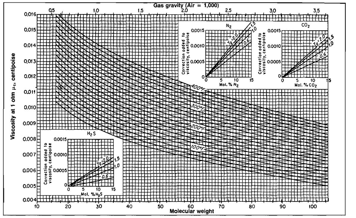
The viscosity at one atmosphere is obtained first from Picture 12 and corrected for nonhydrocarbon impurities if necessary. This viscosity is a function of molecular weight or gravity and temperature only. The correction for pressure is obtained from Picture 13 as a function of reduced pressure and temperature.

An analytical expression for viscosity of hydrocarbon gas was presented by Lee, et al. in 1966. The equation is:
where:
In these equations:
- T = °R;
- μg = cp;
- M = molecular weight and;
- ρg = gm/cm3.
Example 16:
Using both the Carr and Lee methods, calculate the viscosity of a 0,8 gravity gas at a pressure of 2 000 psia and a temperature of 150 °F. The gas contains 10 % H2S and 10 % CO2.
Solution:
Carr Method
From Picture 12:
- μ1 = 0,0111 cp;
- Correction for 10 % H2S = +0,0003;
- Correction for 10 % CO2 = +0,0006.
From Picture 13:
Lee Method
The Lee method does not include a method for correcting for nonhydrocarbon impurities; therefore, the value obtained will be for a pure hydrocarbon gas. However, if the Z-factor used in calculating the gas density has been corrected, the Lee method is valid for sour gases:
It is sometimes convenient to express the viscosity of a fluid as a kinematic viscosity, v. The relationship between viscosity and kinematic viscosity is:
where:
- ρ – is the fluid density.
Gas-Water Systems
In many cases the engineering design of gas production operations will involve natural gas in contact with water. This water may be connate reservoir water or water produced from some other zone. In any event, it is necessary to determine the water contained in the gas in the vapor state, the gas dissolved in the water, and under what conditions of pressure and temperature gas hydrates will be formed.
Solubility of Natural Gas in Water
The solubility of natural gas in water is very low at most pressures and temperatures of interest in gas production engineering. The primary factors affecting the amount of gas that will be evolved from water saturated with the gas depends on pressure, temperature, and solids content of the water. The relationship is illustrated in Picture 14.
The correction factor for salinity may be calculated from:
where:
- Y = salinity of water, ppm;
- X = 3,471/T0,837;
- T = temperature, °F;
- Rsw = gas solubility in brine;
- Rswp = gas solubility in pure water.
Example 17:
Calculate the scf of gas dissolved in a brine containing 50 000 ppm at a pressure of 5 000 psia and a temperature of 200 °F.
Solution:
From Picture 14, Rswp = 20 scf/STB
Solubility of Water in Natural Gas
The solubility of natural gas in water is very low at most pressures and temperatures of interest in gas production engineering. The primary factors affecting the amount of gas that will be evolved from water saturated with the gas depends on pressure, temperature, and solids content of the water. The relationship is illustrated in Picture 14.

The correction factor for salinity may be calculated from:
where:
- Y = salinity of water, ppm;
- X = 3,471/T0,837;
- T = temperature, °F;
- Rsw = gas solubility in brine;
- Rswp = gas solubility in pure water.
Example 17:
Calculate the scf of gas dissolved in a brine containing 50 000 ppm at a pressure of 5 000 psia and a temperature of 200 °F.
Solution:
From Picture 14, Rswp = 20 scf/STB
Solubility of Water in Natural Gas
The amount of water vapor contained in natural gas at various temperatures and pressures must be known in order to relate surface water production to equivalent volumes in the reservoir. The water content is also important in calculations involving hydrate formation. The water content depends on pressure, temperature, and water salinity. Picture 15 shows the mass or weight of fresh water contained in gas as a function of pressure and temperature.
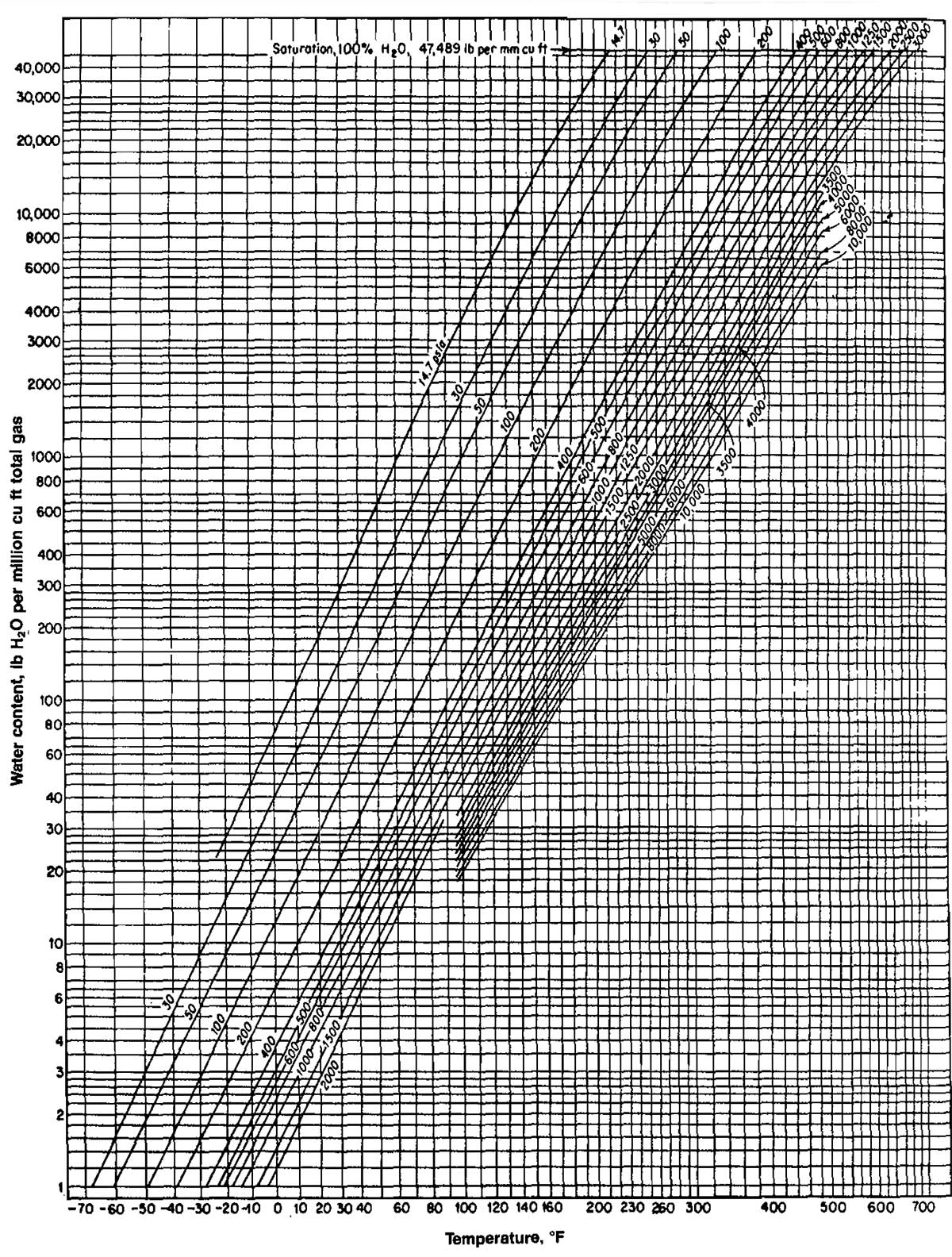
The following equation can be used to correct for water salinity.
where:
- Ws = brine content, lbm/MMscf;
- Wsp = pure water content from Picture 15;
- Y = salinity of water, ppm.
Example 18:
Determine the water content in a natural gas in contact with a 100 000 ppm brine at 3 000 psia and 200 °F.
Solution:
From Picture 15, Wsp = 280 lbm/MMscf
Gas Hydrates
Gas hydrates are crystalline compounds, formed by the chemical combination of natural gas and water under pressure at temperatures considerably above the freezing point of water. In the presence of free water, hydrates will form when the temperature of the gas is below a certain temperature, called the “hydrate temperature”. Hydrate formation is often confused with condensation, and the distinction between the two must be clearly understood. Condensation of water from a natural gas under pressure occurs when the temperature is at or below the dew point at that pressure. Free water obtained under such conditions is essential to the formation of hydrates that will occur at or below the hydrate temperature at the same pressure. Hence, the hydrate temperature would be below, and perhaps the same as, but never above the dew point temperature.
In solving gas production problems, it becomes necessary to define, and thereby avoid, conditions that pro- mote the formation of hydrates. Hydrates may choke the flow string, surface lines, and well testing equipment. Hydrate formation in the flow string would result in a lower value for measured wellhead pressures. In a flow rate measuring device, hydrate formation would result in lower flow rates. Excessive hydrate formation may also completely block flow lines and surface equipment.
Conditions promoting hydrate formation are:
- Gas at or below its water dew point with “free” water present;
- Low temperature, and;
- High pressure.
A further discussion of hydrate formation and prevention is given in Gas Field Operation Problems and Methods to Deal With Them“Gas Production Problems and Methods to Detect Them”.
Gas-Condensate Systems
As the exploration for natural gas is extended to deeper horizons, more reservoirs containing gas condensates are discovered. The gas may be in the gaseous phase at initial reservoir conditions but may condense to form some liquid at some point in the path to the separator.
Engineering design of these production systems requires some understanding of phase behavior. This section deals with the phenomenon of phase change and with methods to calculate these phase changes.
Phase Behavior
Phase behavior is simple for single component systems but becomes more complicated as more components are added to the system. A discussion of the simplest system will lead to an understanding of the more complex systems.
Single Component Fluid. The phase behavior of a fluid can be described by determining its response to pressure and temperature changes. In a liquid the molecules are very close together, but in a gas the molecules are widely separated. Certain forces exist that tend to either confine or disperse the molecules. Confining forces are primarily pressure and molecular attraction. Dispersing forces are kinetic energy and molecular repulsion. The relative magnitudes of the confining and dispersing forces dictate whether the fluid is a liquid or a gas.
An increase in temperature increases the kinetic energy of the molecules and thus the dispersing forces, while an increase in pressure increases the confining forces.
The behavior of a single component fluid can be illustrated graphically on a plot of pressure versus temperature, called a phase diagram. A line joining all of the points where the confining and repelling forces are equal can be plotted. This is a vapor pressure line and is illustrated in Picture 16.
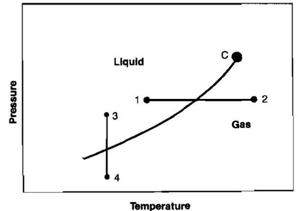
At any point above the vapor pressure line the fluid is a liquid, while below the line the fluid is a gas. At the critical point, Point C, there is no distinction between liquid and gas. A phase change at constant pressure occurs when temperature changes, as illustrated by the path 1-2. A phase change will also occur at constant temperature as pressure is changed (path 3-4).
Multicomponent Fluids. When more than one fluid is present, the difference in molecule size and energy has an influence on the phase change. Picture 17 illustrates the phase diagram for a two-component mixture and Picture 18 shows the phase diagram for a typical hydrocarbon multicomponent mixture.
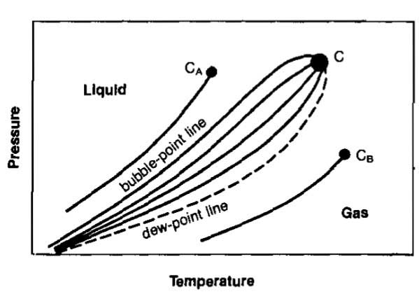
There is no sharp transition from liquid to vapor or from vapor to liquid, but the molecules are able to escape from the liquid or gas at different pressures and temperatures because of molecular attraction. The locus of all points where the first bubble of gas appears in a liquid as pressure and temperature conditions are changed is called the bubble point line.

The locus of all points where the first droplet of liquid appears as the conditions for a gas are changed is the dew point line. The highest pressure at which a gas can exist is called the cricondenbar while the highest temperature at which a liquid can exist is the cricondenthenn.
Separation Process. The two types of separation processes that can occur as pressure or temperature on a fluid changes are called differential and flash or equilibrium. These processes are illustrated in Pictures 19 and 20.
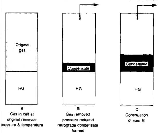
In the differential process the gas is removed from contact with the liquid as it is separated, which means that the composition of the remaining liquid changes constantly.
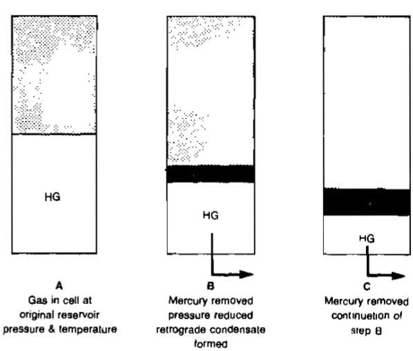
In the flash process the gas remains in contact with the liquid, which means that the process is a constant composition process. Both types of separation, or a mixture of the two, can occur as gas is produced from a reservoir to the separator.
Types of Gas Reservoirs
Reservoirs that yield natural gas can be classified into essentially four categories. These are:
- Dry gas – the fluid exists as a gas both in the reservoir and the piping system. The only liquid associated with the gas from a dry gas reservoir is water. A phase diagram of a dry gas reservoir is illustrated in Picture 21;
- Wet gas – the fluid initially exists as a gas in the reservoir and remains in the gaseous phase as pressure declines at reservoir temperature. However, in being produced to the surface, the temperature also drops, causing condensation in the piping system and separator. This behavior is illustrated in Picture 22;
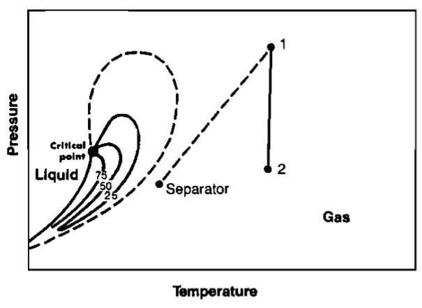
- Retrograde condensate gas – the fluid exists as a gas at initial reservoir conditions. As reservoir pressure declines at reservoir temperature, the dew point line is crossed and liquid forms in the reservoir. Liquid also forms in the piping system and separator. Picture 23 depicts the behavior of a retrograde gas system;
- Associated gas – many oil reservoirs exist at the bubble point pressure of the fluid system at initial conditions. Free gas can be produced from the gas cap of such a system. Gas which is initially dissolved in the oil can also be produced as free gas at the surface. The phase diagram of such a system will depend on the properties of the oil associated with the gas. An example phase diagram is shown in Picture 24.
The fact that hydrocarbon liquids are frequently in contact with natural gas makes it imperative that methods be available to calculate the volumes or masses of each phase and also the composition of each phase existing at various conditions of pressure and temperature. The procedure for accomplishing these calculations is described in the following section.
Flash or Equilibrium Separation Calculations
The phase behavior of an ideal solution can be described by combining the laws of Raoult and Dalton to obtain the quantity of gas and liquid existing at given conditions. Raoult’s Law states that the partial pressure of a component in the gas is equal to the product of the mole fraction of that component in the liquid multiplied by the vapor pressure of the pure component. Raoult’s Law is valid only if both the gas and liquid mixtures are ideal solutions.
The mathematical statement of Raoult’s Law is:
where pj represents the partial pressure of component j in the gas in equilibrium with a liquid of composition xj. The quantity pvj represents the vapour pressure that pure component j would exert at the temperature of interest.
Dalton’s Law can also be used to calculate the partial pressure exerted by a component of an ideal gas mixture:
Raoult’s and Dalton’s Laws both represent the partial pressure of a component in a gas. In the case of Raoult’s Law, the gas must be in equilibrium with a liquid. These laws may be combined by eliminating partial pressure to give an equation that relates the compositions of the gas and liquid phases in equilibrium to the pressure and temperature at which the gas-liquid equilibrium exists, such as:
Equation 34 can be used to calculate the ratio of the mole fraction of a component in the gas to its mole fraction in the liquid. To determine values of yj and xj this equation must be combined with another equation relating these two quantities. Such an equation can be developed through consideration of a material balance on the jth component of the mixture.
Let:
- n represents the total number of moles in the mixture;
- nL represents the total number of moles in the liquid;
- ng represents the total number of moles in the gas;
- zj represents the mole fraction of jth component in the total mixture including both liquid and gas phases;
- xj represents the mole fraction of the jth component in the liquid;
- yj represents the mole fraction of the jth component in the gas;
- zjn represents the moles of the jnth component in the total mixture;
- xjnL represents the moles of the jth component in the liquid, and;
- yjng represents the moles of the jth component in the gas.
A material balance on the jth component results in:
Combination of Equations 34 and 35 to eliminate yj results in:
Since by definition Σxj = 1:
Equations 34 and 35 can also be combined to eliminate xj with the result:
Either equation 36 or 37 can be used to calculate the compositions of the gas and liquid phases of a mixture at equilibrium. In either case a trial-and-error solution is required. The calculation is simplified if one mole of total mixture is taken as a basis so that
and
.
This results in the reduction of Equations 36 and 37 to:
and:
The use of Equation 38 or 39 to predict gas-liquid equilibria behavior is severely restricted since Dalton’s Law is based on the assumption that the gas behaves as an ideal solution of ideal gases. For practical purposes the ideal-gas assumption limits the use of the equations to pressures below about 50 psia.
Raoult’s Law is also based on the assumption that the liquid behaves as an ideal solution. Ideal-solution behavior is approached only if the components of the liquid mixture are very similar chemically and physically.
Another restriction is that a pure compound does not have a vapor pressure at temperatures above its critical temperature. Thus, the use of these equations is limited to temperatures less than the critical temperature of the most volatile compound in the mixture. For example, if methane is a component of the mixture, this method cannot be used at temperatures above -116 °F. These restrictions have led to the use of correlations based on experimental observations. These correlations usually involve the use of the equilibrium ratio K, which is defined as:
From equation 34, it is seen that the K-value is defined by the ratio of the vapor pressure of the component to the system pressure, or:
Substituting this relationship into Equations 38 and 39 results in:
The choice between Equations 40 and 41 is arbitrary; either can be used with equal efficiency. Either equation requires a trial-and-error solution. Normally, successive trial values of
or
are selected until the summation equals one. These equations can be used to calculate the quantity and composition of a mixture by the following procedure. The required data are the feed composition, the pressure and temperature at which the separation is to take place, and K-factors for each component at this pressure and temperature.
- Determine the appropriate K-value for each component at p and T of separation;
Assume a value of
and calculate an assumed value of
from:
for one mole of feed;
Calculate the sum of the mole fractions of all the components using the value of
assumed in Step 2;
If the summation calculated in Step 3 is equal to one, the assumption for
was correct. If not, assume a new value for
and repeat Step 3 until the summation is equal to one.
The xj values calculated in Step 3 represent the composition of the
moles of liquid resulting from the separation. The composition of the
moles of gas can be calculated from:
Step 3 can be modified to calculate the sum of the mole fractions in the gas phase by assuming a value of
and using Equation 41.
Example 19
Calculate the quantity and composition of the gas and liquid phase resulting from a flash separation of the fluid at a pressure of 200 psia and a temperature of 150 °F. Assume that the charts for a convergence pressure of 5 000 psia are applicable.
Solution:
| Component | zj | Kj | yj | |||
|---|---|---|---|---|---|---|
| C3 | 0,61 | 1,520 | 0,484 | 0,505 | 0,501 | 0,761 |
| n-C4 | 0,28 | 0,595 | 0,351 | 0,334 | 0,337 | 0,201 |
| n-C5 | 0,11 | 0,236 | 0,178 | 0,158 | 0,162 | 0,038 |
| 1,00 | 1,013 | 0,997 | 1,000 | 1,000 |
Since Σxj = 1 for
= 0,42, this means that 42 % of the total feed is in the gas phase and 58 % in the liquid phase at 200 psia and 150 °F. Also, for example, 50,1 % of the liquid phase is C3 and 76,1 % of the gas phase is C3.
The previous equations can also be used to determine bubble point and dew point pressures of a mixture at a given temperature. At the bubble point, the amount of gas is negligible and:
and:
The bubble point or dew point pressures can be calculated by trial-and-error by assuming various pressures and determining the pressure that will produce K-values satisfying Equations 42 or 43.
The following relationships will aid in determining the bubble point or dew point.
If Σ zjKj and
are both > 1, p is between pb and pd.
- If Σ zjKj < 1, p > pb.
If
Example 20:
Determine the bubble point pressure of the following mixture at a temperature of 150 °F.
Solution:
From the previous example we know that the bubble point pressure is greater than 200 psia. As a first guess, use pb = 250 psia.
Trial 1 (pb = 250 psia)
| Component | zj | Kj | zjKj |
|---|---|---|---|
| C3 | 0,61 | 1,270 | 0,775 |
| n-C4 | 0,28 | 0,500 | 0,140 |
| n-C5 | 0,11 | 0,203 | 0,022 |
| 1,00 | 0,937 |
The assumed pressure is greater than the bubble point pressure since ΣzjKj < 1.
Trial 2 (pb = 220 psia)
| Component | zj | Kj | zjKj |
|---|---|---|---|
| C3 | 0,61 | 1,490 | 0,909 |
| n-C4 | 0,28 | 0,580 | 0,162 |
| n-C5 | 0,11 | 0,230 | 0,025 |
| 1,096 |
The fact that ΣzjKj > 1 implies that 220 psia is below the bubble point pressure. By linear interpolation, select the pressure for the third trial as 230 psia.
Trial 3 (pb = 230 psia)
| Component | zj | Kj | zjKj |
|---|---|---|---|
| C3 | 0,61 | 1,350 | 0,824 |
| n-C4 | 0,28 | 0,534 | 0,150 |
| n-C5 | 0,11 | 0,223 | 0,025 |
| 0,099 |
The bubble point pressure is therefore 230 psia at a temperature of 150 °F.
Determination of Equillibrium Ratios
In order to apply the methods described in the preceding section, it is necessary to have access to K-values for each component as a function of pressure and temperature. The most widely used method of determining K-values is to use the experimentally determined charts published by the NGPSA 9. The problem with using these charts is that the convergence pressure, pk, must be known in order to select the appropriate chart. At relatively low pressures the K-values are almost independent of convergence pressure, but for separation pressures approaching convergence pressure, they are very sensitive to convergence pressure. The determination of the proper convergence pressure to use for a given system is iterative.
A suggested procedure is:
Estimate a value for convergence pressure,
Read the K-values for each component from the charts prepared at
- Perform a flash calculation using the K-values from Step 2. This gives the liquid composition.
- Identify the lightest hydrocarbon component in the liquid phase which comprises at least 0,001 mole fraction; that is, xj ≥ 0,001. This will usually be C1 or C2 for gas condensate systems.
- Calculate the weight average critical temperature for the remaining heavier components in the liquid phase. These remaining heavier components represent a pseudo-heavy component in the pseudo binary system.
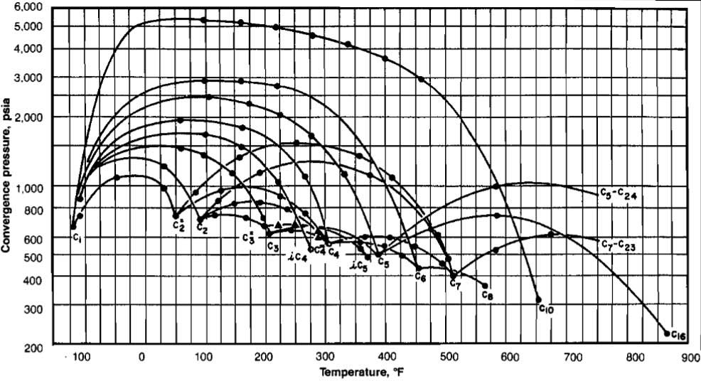
- Enter Picture 25 at the critical temperature calculated in Step 5 and determine which actual hydro carbon component has a critical temperature closest to the pseudo-heavy component. If the value is between two real components, interpolation is required.
Trace the critical locus between the light and pseudoheavy component to the separation temperature and read the convergence pressure pk at this point. If pk ≠
from Step 1, set
and go to Step 2. Repeat until
K-Values from Equations of State
Equilibrium ratios may be defined in tenus of the fugacity of the component in a mixture. The fugacity, f, is a thermodynamic quantity defmed in tenus of the change in free energy in passing from one state to another. It has been shown that the fugacity of a component in a phase of a mixture is equal to the fugacity of that component in the same phase in the pure state multiplied by the mole fraction of the component in the mixture.
That is, for the gas and liquid phases:
If the phases are in equilibrium, the fugacities of a component in the liquid and gas phases are equal, or:
or:
Therefore, the K-values can be approximated if the fugacity of each component can be calculated at a given pressure and temperature. This can be accomplished by the use of an equation of state, such as the Soave-Redlich-Kwong equation described earlier. The fugacity coefficient of a component in a mixture is given by:
where:
The values for Z, A, B, and α are calculated by Equations 22, 23, 24, and 25, respectively. The xj represents either the liquid or gas mole fraction.
The use of an equation of state to calculate phase behavior involves numerous calculations and is usually applied only by utilization of a computer. Some simplified programs have been published for use with hand calculators by Weber.
Adjustment of Properties for Condensate Mixtures
In many cases the properties of the total well or reservoir fluid will not be measured, but the gas and condensate properties after separation will be known. Many reservoir and piping system calculations require properties such as specific gravity for the reservoir or well fluid. Methods for making the calculations are given below.
Specific Gravity of Mixtures. By forming a molal balance on the separator gas and liquid effluents, the following equation can be derived for calculating the gravity of a mixture:
where:
- γgm = specific gravity of the mixture (air = 1);
- γg = specific gravity of the separator gas;
- γo = specific gravity of the condensate;
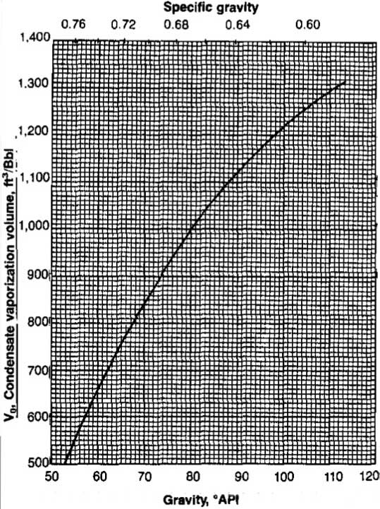
- Vo = condensate vaporizing volume, and;
- R = producing gas-condensate ratio.
The condensate specific gravity is related to the API gravity by:
Vo is obtained from Picture 26 for cases in which γo is measured at a high pressure separator.
If γo is measured at stock tank conditions, the value of Vo depends on separator pressure and is obtained from Picture 27.
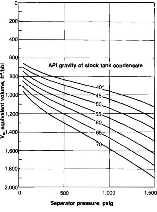
Example 21:
Calculate the specific gravity of a reservoir gas given the following:
- γg = 0,65;
- γo from S. T. = 0,78 (50° API);
- R = 30 000 scf/STB;
- Separator pressure = 900 psig.
Solution:
From Picture 27, Vo = 1 110 scf/STB
Equation 46 can be used to calculate the specific gravity of a gas containing water if the dry gas gravity and water content are known. The liquid vaporizing volume for water is:
To calculate Rw in scf/STB from the water content in lbm/MMscf, use: