Exploring Hybrid Representation for the Attenuation Factor

Learn how hybrid representation techniques are applied using Fock’s contour integral to analyze the attenuation factor W(ξ, h, h₀).

In this article we use a Fock’s contour integral representation for the attenuation factor W(ξ, h, h₀). As shown in Understanding Parabolic Approximation in Wave Propagation: Analytical Methods and Applications“Parabolic Approximation to the Wave Propagation”, both the contour integral representation and the expansion over the set of eigenfunctions of the continuous spectrum are equivalent in representing the attenuation factor W(ξ, h, h₀) in the absence of random inhomogeneities of the refractive index. From practical point of view, in a deterministic problem the manipulations with a contour integral are a bit less cumbersome than eigenfunctions of the continuous spectrum, since the latter contains terms, such as waves χ^–(t, h) coming from infinity that produce a negligible contribution to the integral for positive ξ in the absence of random fluctuations.

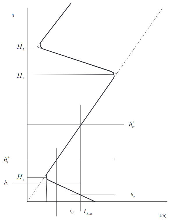
We consider a slightly more general case of the M-profile for the hybrid ray-mode representation, as shown in Figure 1.

Fig. 1 Smooth M-profile for a two-channel model of refractivity

The contour integral for the attenuation factor W(ξ, h, h₀) can be written as:

W (ξ, h, h_{0}) = \sqrt{\frac{ξ}{π}} e^{- j π / 4} \int_{C} K (h, h_{0}, t) e^{j ξ t} d t . E q . 1

The function K(h, h₀, t) satisfies the equation:

\frac{d^{2}}{d h^{2}} K + [U (h) - t] K = δ (h - h_{0}) E q . 2

and the conditions:

{(\frac{d K}{d h} + q K)}_{h = 0} = 0, E q . 3

\frac{d}{d h} \arg K_{h \to \infty} > 0,

where q = jmZ and Z is a surface impedance of the interface h = 0. The integration contour embraces singularities of the integrand lying in the first quadrant. The precise form of K depends on the shape of the profile U(h) and the relative values h, h₀, H_s and H_i. If both the transmitter and the receiver are within the lower inversion layer, i. e. h₀ < h < H_s, then K takes the form:

K (h, h_{0}, t) = - \frac{[f_{2} (h_{0}, t) + R_{g} f_{1} (h_{0}, t)] \cdot [f_{1} (h, t) + R \cdot f_{2} (h, t)]}{W (f_{1}, f_{2}) [1 - R (t) R_{g} (t)]}, E q . 4

where f₁ and f₂ are the independent solutions of uniform equation (2) specified within 0 < h < H_s, and:

W = f_{1} \frac{d f_{2}}{d h} - f_{2} \frac{d f_{1}}{d h} . E q . 5

The values R_g and R are defined as:

R_{g} = - \frac{f_{2}^{'} (0, t) + q f_{2} (0, t)}{f_{1}^{'} (0, t) + q f_{1} (0, t)}, E q . 6

R = - \frac{f_{1}^{'} (H_{s}, t) - f_{1} (H_{s}, t) \frac{φ_{1}^{'} (H_{s}, t) + R_{i} \cdot φ_{2}^{'} (H_{s}, t)}{φ_{1} (H_{s}, t) + R_{i} \cdot φ_{2} (H_{s}, t)}}{f_{2}^{'} (H_{s}, t) - f_{2} (H_{s}, t) \frac{φ_{1}^{'} (H_{s}, t) + R_{i} \cdot φ_{2}^{'} (H_{s}, t)}{φ_{1} (H_{s}, t) + R_{i} \cdot φ_{2} (H_{s}, t)}} E q . 7

R_{i} = \frac{φ_{1}^{'} (H_{i}, t) - φ_{1} (H_{i}, t) \cdot \frac{ψ_{1}^{'} (H_{i}, t)}{ψ_{1} (H_{i}, t)}}{φ_{2}^{'} (H_{i}, t) - φ_{2} (H_{i}, t) \cdot \frac{ψ_{1}^{'} (H_{i}, t)}{ψ_{1} (H_{i}, t)}} E q . 8

The functions φ₁ and φ₂ are independent solutions of the uniform equation (2) for H_s < h < H_i, and ψ₁ is the solution for h > H_i which satisfies the condition:

\frac{d}{d h} \arg ψ_{1} > 0 with h \to \infty . E q . 9

The derivative sign f^′ in Eqs. (6)–(8) means the derivative over the h-variable. Apparently, R_g, R and R_i can be regarded as the reflection coefficients at h = 0, h = H_s and h = H_i, respectively.

Now we can get to the hybrid representation of the received field, as manifested in the beginning of this article. As a first step toward implementing this program we will express the factor (1-R_iR_g)^-1 in terms of a partial geometric series:

{(1 - R_{i} R_{g})}^{- 1} = 1 + \sum_{n = 1}^{N} {(R_{i} R_{g})}^{n} + \frac{{(R_{i} R_{g})}^{N + 1}}{1 - R_{i} R_{g}} E q . 10

and substitute Eq. (10) into the integral (1):

W (ξ, h, h_{0}) = \sqrt{\frac{ξ}{π}} e^{- j π / 4} \int_{C} d t e^{j ξ t} W^{- 1} (f_{1}, f_{2}) \cdot \{F_{1} (h_{0}, t) [f_{1} (h, t) + R f_{2} (h, t)] + \sum_{n = 1}^{N} {(R R_{g})}^{n} F_{1} (h_{0}, t) [f_{1} (h, t) + R f_{2} (h, t)] + \frac{{(R R_{g})}^{N + 1} F (h, h_{0}, t)}{1 - R R_{g}}\} E q . 11

Here:

F_{1} (h_{0}, t) = f_{2} (h_{0}, t) + R_{g} f_{1} (h_{0}, t),

F_{1} (h, h_{0}, t) = - K (h, h_{0}, t) W (f_{1}, f_{2}) (1 - R R_{g}) E q . 12

and N is an arbitrary integer whose choice is dictated by the length of the propaga- tion path. It represents the maximum number of reflections from the upper “boundary” h = H_i to be taken into account.

If there is no elevated M-inversion (cf. the dashed profile in Figure 1), the attenuation function W(ξ, h, h₀) would take the form:

W (ξ, h, h_{0}) = \sqrt{\frac{ξ}{π}} e^{- j π / 4} \int_{C} d t e^{j ξ t} \frac{F_{1} (h_{0}, t) [f_{1} (h, t) + R_{s} f_{2} (h, t)]}{W (f_{1}, f_{2}) (1 - R_{s} R_{g})}, E q . 13

where R_s denotes the reflection coefficient at the “upper wall” h = H_s of the surface duct, i.e:

R_{s} = - \frac{f_{1}^{'} (H_{s}, t) - f_{1} (H_{s}, t) \frac{φ_{1}^{'} (H_{s}, t)}{φ_{1} (H_{s}, t)}}{f_{2}^{'} (H_{s}, t) - f_{2} (H_{s}, t) \frac{φ_{1}^{'} (H_{s}, t)}{φ_{1} (H_{s}, t)}} E q . 14

Of the two independent functions above H_s, i. e. φ₁ and φ₂, only φ₁ will remain because of the “new” condition:

\frac{d}{d h} \arg φ > 0 with h > H_{s} . E q . 15

To isolate the set of eigenwaves of a solitary surface duct from the solution (11), we multiply and divide the first term of Eq. (11) by the “resonant denominator” of Eq. (13), i. e., (1-R_sR_g), and represent R as:

R = R_{s} - R_{i} \frac{Λ_{1} + R_{s} Λ_{2}}{1 + R_{i} Λ_{2}} = R_{s} - R_{i} v E q . 16

with:

\begin{matrix} Λ_{1} = \frac{f_{1}^{'} (H_{s}, t) \cdot φ_{2} (H_{s}, t) - f_{1} (H_{s}, t) \cdot φ_{2}^{'} (H_{s}, t)}{f_{2}^{'} (H_{s}, t) \cdot φ_{1} (H_{s}, t) - f_{2} (H_{s}, t) \cdot φ_{1}^{'} (H_{s}, t)} \\ Λ_{2} = \frac{f_{2}^{'} (H_{s}, t) \cdot φ_{2} (H_{s}, t) - f_{2} (H_{s}, t) \cdot φ_{2}^{'} (H_{s}, t)}{f_{2}^{'} (H_{s}, t) \cdot φ_{1} (H_{s}, t) - f_{2} (H_{s}, t) \cdot φ_{1}^{'} (H_{s}, t)} \end{matrix} E q . 17

Now consider the function g(h, t) defined as the solution of:

\frac{d^{2}}{d h^{2}} g + [U_{1} (h) - t] g = 0 E q . 18

with the conditions:

{(\frac{d g}{d h} + q g)}_{h = 0} = 0, E q . 19

g (H_{s}, t) = C (t) φ_{1} (H_{s}, t) E q . 20

where U₁(h) corresponds to the dashed M-profile of Figure 1. We can obtain that:

1 - R_{s} R_{g} = \frac{{(\frac{d g}{d h} + q g)}_{h = 0}}{g (0, t) [f_{1}^{'} (0, t) + q f_{1} (0, t)]} \cdot [f_{1} (0, t) - \frac{f_{1}^{'} (H_{s}, t) - f_{1} (H_{s}, t) \frac{φ_{1}^{'} (H_{s}, t)}{φ_{1} (H_{s}, t)}}{f_{2}^{'} (H_{s}, t) - f_{2} (H_{s}, t) \frac{φ_{1}^{'} (H_{s}, t)}{φ_{1} (H_{s}, t)}} f_{2} (0, t)] E q . 21

and hence Eq. (19) is equivalent to the characteristic equation 1-R_sR_g = 0 specifying the modes of the surface duct. Further, we bring the integrand of Eq. (11) to the form:

\frac{F_{1} (h_{0}, t) [f_{1} (h, t) + R_{s} f_{2} (h, t)]}{1 - R_{s} R_{g}} - \frac{F_{1} (h_{0}, t) R_{i} v f_{2} (h, t)}{1 - R_{s} R_{g}} - \frac{F (h, h_{0}, t) R_{s} R_{g}}{1 - R_{s} R_{g}} + \sum_{n = 1}^{N} F (h, h_{0}, t) R_{g}^{n} [R_{s}^{n} + \sum_{p = 1}^{n} (\begin{matrix} n \\ p \end{matrix}) {(- 1)}^{p} R_{s}^{n - p} R_{i}^{p} v^{p}] + \frac{{(R R_{g})}^{N + 1} F (h, h_{0}, t)}{1 - R R_{g}} E q . 22

with

(\begin{matrix} n \\ p \end{matrix})

being binominal coefficients, and express the first integral as a sum of the residues at

t = {\hat{t}}_{n},

or the zeros of the equation 1-R_sR_g = 0 (the bar serves to indicate their distinction from the roots of 1-RR_g = 0).

Representing (1-R_sR_g)^-1 in the second and third term as another partial geometric series, gen- erally speaking with a number of terms different from Eq. (10), we assemble similar terms and arrive at:

W (ξ, h, h_{0}) = \sqrt{\frac{ξ}{π}} e^{- j π / 4} (W_{01} + T_{2} + T_{3} + T_{4}) E q . 23

where term W₀₁ represents the sum of the normal modes of the surface duct:

W_{01} = 2 π j \sum_{n = 1}^{\infty} \exp (j {\hat{t}}_{n} ξ) \frac{d {\hat{t}}_{n}}{d q} \frac{g (h, {\hat{t}}_{n})}{g (0, {\hat{t}}_{n})} \frac{g (h_{0}, {\hat{t}}_{n})}{g (0, {\hat{t}}_{n})} E q . 24

and:

T_{2} = - \int_{C} d t e^{j ξ t} W^{- 1} (f_{1}, f_{2}) F_{1} (h_{0}, t) R_{i} v \cdot f_{2} (h, t), E q . 25

T_{3} = \sum_{n = 1}^{N} \int_{C} d t \frac{e^{j ξ t}}{W (f_{1}, f_{2})} R_{g}^{n} \cdot [F (h, h_{0}, t) \sum_{p = 1}^{n} (\begin{matrix} n \\ p \end{matrix}) {(- 1)}^{p} R_{s}^{n - p} R_{i}^{p} v^{p} - F_{1} (h_{0}, t) R_{i} v R_{s}^{n} f_{2} (h, t)], E q . 26

T_{4} = \int_{C} d t \frac{e^{j ξ t}}{W (f_{1}, f_{2})} [\frac{F (h, h_{0}, t)}{1 - R R_{g}} {(R R_{g})}^{N + 1} - \frac{F_{2} (h, h_{0}, t)}{1 - R_{s} R_{g}} {(R_{s} R_{g})}^{N + 1}] E q . 27

where:

F_{2} (h, h_{0}, t) = F_{1} (h_{0}, t) [f_{1} (h, t) + R_{s} f_{2} (h, t)] . E q . 28

The term T₂ can be interpreted as the field arriving at the observation point due to a single reflection from the elevated inversion while T₃ is a set of waves multiply reflected between the boundaries h = H_i, h = H_s, and h = 0. T₄ is a remainder term whose smallness will be secured by the proper choice of N for every specific separa- tion from the source. It should be emphasized that in bringing Eq. (11) to the form of Eq. (23) we made no approximation, and hence Eq. (23) is an exact representation of the field in the structure analysed (to be more precise, it is exact in the same sense as the initial formula Eq. (1), which itself corresponds to a parabolic equation approximation).

The set of normal modes associated with the surface duct, the entire infinite spectrum, has been separated from Eq. (1) solely by transforming the integrand (4). The fields given by T₂ and T₃ so far cannot be interpreted in the ray optical form, since rays appear only at the stage of asymptotic evaluation of the integrals.

As for the numerical truncation of the modal series, the question seems almost trivial, since in the absence of a reflecting upper wall the higher-order modes are evanescent and their respective eigenvalues have the ordering:

I m {\hat{t}}_{n + 1} > I m {\hat{t}}_{n} .

As observed from Eqs. (25) and (26), the integrands T₂ and T₃ contain no singularities. Depending on the number of significant saddle points, each of these integrals splits into several terms representing waves which are radiated either up or down from the transmitting antenna. Further along the path, they are reflected from the boundaries h = 0, h = H_s and h = H_i to arrive at an observation point along some of the ray trajectories of Figure 2.

For example, T₂ splits into two terms, each corresponding to a wave that is reflected once from the elevated layer. The first leaves the source in an upward direction, reaches a reflection point in the upper layer, and comes to the observation point along the ray 1, Figure 5.7. Another emerges downwards from the source downward, undergoes reflections from the earth’s surface and the elevated layer, and arrives at the observation point along trajectory 2, Figure 2.

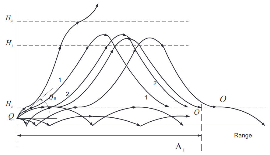
Ray trajectories — Fig. 2 Schematic of the ray trajectories in the structure shown in Figure 1; Λ_i is the maximum range attainable through a single reflection from the upper layer

The different components of the angular spectrum of waves excited by the transmitter dipole are subject to a kind of spatial “filtration” in the nonuniform troposphere. We can define the critical angle θ₀ as the angle at which the ray QO^′ emerging from the source turns at the height h = H_s, as shown in Figure 2. The rays with departure angles θ < θ₀ are trapped by the surface duct; those with θ > θ₀ leave it freely.

The ray with θ = θ₀+δ, δ → 0 comes back to earth, upon reflection from the elevated layer, at the maximum range attainable to a single reflection from the elevated layer, we define this range as ξ_1m. Real rays arriving at greater distances than ξ_1m can do so only through a higher number of reflections from the “boundaries” h = H_i, h = 0 and h = H_s. Generally, each group of rays of a given reflection multiplicity, l, has its own “horizon”, i. e. the limiting distance still corresponds to real stationary points in the integrand of T₂ (for l = 1) and/or T₃ (l > 1). It is in the vicinity of the lth horizon that the contribution of l times the reflected wave is the highest.

Indeed, the grazing angle with respect to the elevated layer assumes the lowest possible value when the observation point is near the horizon. As a result, one can distinguish, along the path, characteristic zones of the “first hop” (i. e. near n = ξ_1m where is the dominant contribution to T₂+T₃+T₄, for the N terms in T₃, only those with l ≤ N “work“). Moving beyond the lth horizon, an observer finds himself in an umbral zone where the field of the l+1 hop has not yet formed while that of the lth hop can no longer propagate except by diffraction. The magnitude of this diffractional field is determined by the small contribution of complex rays corresponding to the complex stationary points of T₂ and/or T₃, but mainly by the value of the remainder integral T₄. For evaluating this latter it seems convenient to represent it as:

T_{4} = T_{41} + T_{42} E q . 29

with:

T_{41} = \int_{- \infty}^{\infty} d t \frac{e^{j ξ t} F_{1} (h_{0}, t)}{1 - R_{s} R_{g}} [f_{1} (h, t) + f_{2} (h, t) \frac{R^{N + 1} - R_{s}^{N + 1}}{R^{N} - R_{s}^{N}}] R_{g}^{N + 1} R (R^{N} - R_{s}^{N}), E q . 30

T_{42} = \int_{- \infty}^{\infty} d t \frac{e^{j ξ t} F_{1} (h_{0}, t) {(R_{s} R_{g})}^{N + 1}}{(1 - R_{s} R_{g}) (1 - R R_{g})} [f_{2} (h, t) + f_{1} (h, t) \frac{1}{R_{s}}] R (R - R_{s}) . E q . 31

As can be seen, T₄₁ is the contribution of waves N+1 times reflected from the upper layer, and hence it should be small near the horizon of l ≤ N-reflected waves.

The number of reflections, N, which are to be taken into account at a specific distance from the transmitter can be estimated as follows: Let us assume for simplicity that the reflection coefficient R_i depends on the grazing angle θ as:

\begin{matrix} R_{i} (θ) = 1, θ \leq θ_{0} \\ R_{i} (θ) = 0, θ > θ_{0} \end{matrix} E q . 32

where θ is with respect to the lower edge of the layer, r_i = a+Z_i. Consider the field T_N due to reflections from the upper layer, for h = h₀ = 0 and

ξ ≅ 2 \sqrt{H_{i}}

(i. e., near the horizon of singly reflected waves), i. e.:

T_{N} ~ e x p [j ξ t + j \frac{4}{3} N {(H_{i} - t)}^{3 / 2} - j \frac{4}{3} N {(- t)}^{3 / 2}] . E q . 33

The saddle point of Eq. (33) is:

t^{(N)} = - H_{i} \frac{{(N^{2} - 1)}^{2}}{4 N^{2}} . E q . 34

Recalling the relation between the grazing angle and t, i. e.:

\cos θ = \frac{k a + m t}{k r_{i}} E q . 35

and the fact that real saddle points of real rays satisfy the inequality:

t \leq m i n (h, h_{0}) E q . 36

we can obtain from Eq. (35) an estimate at t → 0 for the grazing angle θ of N times the reflected waves:

θ_{m i n}^{(N)} ≅ {(\frac{2 H_{i}}{a})}^{1 / 2} \frac{N^{2} + 1}{2 N} . E q . 37

To have R_i(θ_min) ≠ 0, it is necessary that:

{(\frac{2 H_{i}}{a})}^{1 / 2} \frac{N^{2} + 1}{2 N} \leq θ_{0} . E q . 38

The order of magnitude of θ₀ is 10^–2, and that of (2H_i/a)^1/2 ≅ 5·10^-3 to 10^-2, whence the number of terms to be retained in Eq. (23) near the horizon l = 1 is N = 1–3.

We leave evaluation of the magnitude of term T₄₂ in Eq. (31) until the next section, noting here that its contribution cannot be described in pure ray optical terms. In fact this term describes a peculiar physical effect of secondary excitation of the surface (evaporation) duct.

A better illustration of the relative importance of the different terms in Eq. (23) can be achieved through numerical analysis. Figure 3 represents the calculated attenuation function for f = 10 GHz in a two-channel structure of the refractivity. The surface M-inversion is characterised by Z_s = 9 m, ΔM = M(0)-M(Z_s) = 2 M-units. The elevated M-inversion lies at the height Z_i = 500 m and has been approximated with a discontinuity ΔM_i = 10 M-units of no thickness (i. e., Z_k = Z_i).

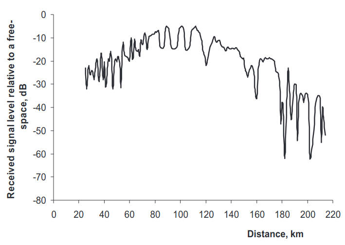
Signal strength — Fig. 3 Calculated signal strength level for a two-channel system at frequency 10 GHz: Z_s = 9 m, ΔM = 2 M-units, Z_i = 500 m and ΔM_i = 10 M-units

An approximation like this obviously results in an overestimated value of the reflection coefficient R_i(t). The heights of the transmitting and receiving antennas are z₀ = 8,5 m and z = 5 m, respectively, apparently both inside the evaporation duct. The normalised impedance q of the earth’s surface is assumed to have a value corresponding to that of sea water: Req = 6, Im q = 94. The calculated imaginary part of the first-mode eigenvalue is found to be Im t₁ = 0,4. For a given combination of the antenna heights the optical horizon would be at ≈ 20 km. As observed from Figure 3, there is a region beyond that horizon (extending to about 60 or 70 km) where the field level is determined by the lower-order mode of the surface duct alone. Further along the path, the contribution of waves reflected from the elevated layer becomes substantial. In the zone of the first hop (i. e. 60 km ≤ x ≤ 200 km) the maximum field strength becomes close to the free space level. The remainder term T₄ reaches a –40 dB level near distance 200 km with N = 1.

The mechanism of the radio wave propagation in the above two-channel system can be summarised as follows. At relatively smaller distances from the transmitter the dominant contribution to the received signal strength comes from evaporation duct propagation alone. Further along the path, the waves, departing with angles exceeding the critical angle θ₀ and reflected by the elevated M-inversion, contribute to the received field at an appropriate distance of the single hop. These waves interfere with each other as well as with the waves propagating through the evaporation duct producing the deep fades caused by large phase difference. For example, in Figure 3, the deepest fades are observed in the range 60–100 km where the wave propagating through the evaporation duct and superposition of the waves reflected from the elevated M-inversion are comparable in amplitude. Then, along the distance, the field reflected from the elevated M-inversion takes over and provides the major contribution to the received field strength.

Secondary Excitation of the Evaporation Duct by the Waves Reflected from an Elevated Refractive Layer

Referring to the discussion in the previous section and Figure 2, we state that the rays with departure angles from the source less than critical angle θ₀ are trapped in the surface duct, those with θ > θ₀ leave it freely. We also note that rays with θ > θ₀ reach the observation point at the distances ξ < ξ_1max. At distances greater than the horizon of first hop (ξ_1max, single reflection) there are no single reflected rays launched at the angles of departure θ > θ₀. Hence, between the first and second hop there is a range of distances where the receiving field is formed by another mechanism represented by term T₄₂ in Eq. (31) and evaluated in this section.

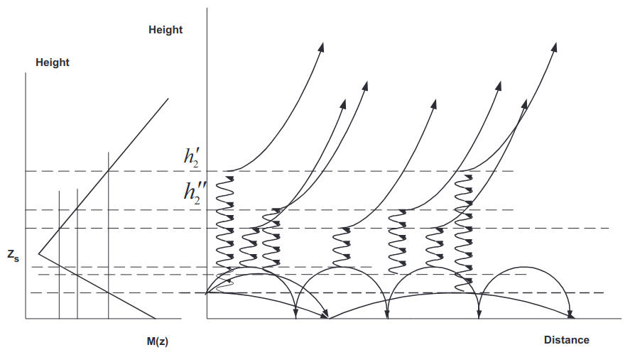
Consider the range of distances ξ ≥ ξ_1max concentrated on trapped waves/rays. The trapped waves with departure angles θ < θ₀ turn inside the surface duct, as shown in Figure 3. Since the potential barrier is finite the trapped waves can leak to the space above the surface duct as shown schematically in Figure 4, their respective phases are complex due to the leaking mechanism distributed along the distance. The field created by these waves in the space above the surface duct can be imagined as a cluster of rays distributed along the distance and sliding along the tangents to circles of radius r = a+h₂, where the height h₂ is given by the relation 2m² 10^–6 M(h₂) = t for h₂ > Z_s, where t is a dimensionless “energy” corresponding to the angle θ.

Penetration of waves — Fig. 4 Schematic diagram of the penetration of “leaked” modes through the potential barrier in an evaporation duct

In evaluating the maximum magnitude of T₄₂ and therefore the impact from sec- ondary excitation at ξ ≥ ξ_1max we shall set N = 1. Taking into account that the observation point lies within the surface layer, we will represent the integral (31) as a sum of residues at the zeros of 1–R_sR_g = 0.

Using Eq. (16) we can isolate the coefficient of reflection from the upper boundary of the surface duct R_s in R and present the denominator of Eq. (31) in the form:

(1 - R R_{g}) (1 - R_{s} R_{g}) = {(1 - R_{s} R_{g})}^{2} [1 - \frac{R_{i} R_{g} v}{1 - R_{s} R_{g}}] . E q . 39

The term v may be interpreted as a coupling factor between the lower and upper ducts. For low attenuating modes (Im t_n ≪ 1) it can be estimated as:

v (t_{n}) \approx e x p (- \frac{4}{3} \frac{μ + 1}{μ} t_{n}^{3 / 2}) E q . 40

where μ = |dU/dh| is a gradient of profile U(h) for 0 < h < H_s. The greater Re t_n the lower is the turning height h₁, the lesser the amount of leaking from the surface duct and, in accordance with a reciprocity theorem, such waves are harder to generate by a source distributed across the reflective layer but outside the surface duct.

To finish evaluation of T₄₂, we write a partial geometric series for (1-R_sR_g)^-1 (1-RR_g)^-1 with the help of formula (39), namely:

{(1 - R_{s} R_{g})}^{- 1} {(1 - R R_{g})}^{- 1} = {(1 - R_{s} R_{g})}^{- 2} \cdot [1 + \sum_{p = 1}^{P - 1} \frac{{(- R_{i} R_{g} v)}^{p}}{{(1 - R R_{g})}^{p}} + \frac{{(- R_{i} R_{g} v)}^{P}}{(1 - R R_{g}) {(1 - R_{s} R_{g})}^{P - 1}}] E q . 41

and substitute it in Eq. (31).

Now we restrain the evaluation by the first term of the expansion (41) using the same arguments of angular filtration as in the previous section. Then we assume that H_i-H_s ≫ 1 and a/H_i·10^-6 ΔM ≪ 1, where ΔM = M(z = 0)-M(Z_s) is the M-deficit of the surface duct. Therefore, we assume that the waves reflected from the elevated refractive layer can be regarded as a plain waves on their arrival at the level of the surface duct, and the horizons of departure of the leaked waves h₂ in Figure 4 are not to too different from H_s compared with H_i, i. e., max(h₂)/H_i ≪ 1. This allows us to use the same magnitude of the reflection coefficient |R_i(t)| ≈ |R_i(0)| for all rays from the cluster of leaking waves, expanding the amplitude and phase of the reflection coefficient into a series over powers of t. Taking into account that the observation point lies within the surface layer, we will represent the integral (31) as a sum of residues at the zeros of (1-R_sR_g)² = 0.

T_{42} ≅ 2 π j |R_{i} (0)| \exp \{j \frac{4}{3} [{(H_{i} - H_{s})}^{3 / 2} + δ (0)]\} \sum_{s = 1}^{S} \exp (j ξ {\hat{t}}_{s}) (1 + q) v ({\hat{t}}_{s}) {(\frac{d {\hat{t}}_{s}}{d q})}^{2} \cdot \{\frac{g (h, {\hat{t}}_{s})}{g (0, {\hat{t}}_{s})} \frac{g (h_{0}, {\hat{t}}_{s})}{g (0, {\hat{t}}_{s})} [\frac{v^{'} ({\hat{t}}_{s})}{v ({\hat{t}}_{s})} + j ξ + 3 g^{- 1} (0, {\hat{t}}_{s}) \frac{\partial g (0, {\hat{t}}_{s})}{\partial {\hat{t}}_{s}} + \frac{d {\hat{t}}_{s}}{d q} \frac{\partial}{\partial {\hat{t}}_{s}} {(\frac{d {\hat{t}}_{s}}{d q})}^{- 1}] + \frac{\partial}{\partial {\hat{t}}_{s}} [\frac{g (h, {\hat{t}}_{s})}{g (0, {\hat{t}}_{s})} \frac{g (h_{0}, {\hat{t}}_{s})}{g (0, {\hat{t}}_{s})}]\} . E q . 42

Here S is the number of modes trapped in the surface duct.

Equation (42) provides an estimate of the secondary excitation of the surface duct by a limited number of the modes of the surface duct, “trapped”, from the point of view of geometrical optics but, in fact, “leaking” from the duct along the distance of propagation due to the finite thickness of the potential barrier in U(h). These waves, then being reflected from the elevated M-inversion, reach the surface duct from above and “leak” back into the wave guide reproducing itself in the surface duct. Of course, the symmetry in the secondary excitation of the surface duct relies on the uniformity of the refractive index in the horizontal plane along the distance. Analysing Eq. (42) we may note that for the shorter wavelength λ of the electromagnetic radiation, the trapping condition of the surface duct becomes stronger and leaking of the trapped modes is reduced, as is the attenuation of the ducted field with distance. This leads to an even smaller contribution from the secondary excited field described by term T₄₂, Eq. (42).

Increase in the wavelength λ leads, on the one hand, to a greater attenuation of the ducted field and stronger leaking of the trapped modes from the duct and, on the other hand, to better conditions for reflection from the elevated layer and stronger secondary excitation of the surface duct. The major contribution to the secondary guided field is from the modes with |Re t_n| ≪ 1. These modes have relatively high attenuation compared with deeply trapped modes, however they still provide a significant contribution at smaller distances from the source and, being reflected from the elevated layer, at distances ξ ≥ ξ_1max. Evaluating this result numerically, we have found that the secondary guided field given by Eq. (42) may reach a maximum level of –50 dB relative to a free space condition with ideal reflection from the elevated layer, |R_i| = 1.

The rather exotic though observable situation is shown in Figure 5 where we have extremely strong elevated M-inversion and surface-based evaporation duct simultaneously. Here Z_s = 18 m, ΔM = M(0) – M(Z_s) = 6 M-units, Z_s = 500 m, Z_k = 600 m, ΔM_s = 60 M-units. The calculation was performed for radio frequency f = 3 GHz and the following combination of antenna heights:

z₀ = 16 m;
z = 10 m and 50 m, respectivly.

Figure 5 shows that the field reflected from elevated M-inversion dominates at distances of the order of the reflection cycle length Λi despite there being lots of trapped modes of the elevated duct.

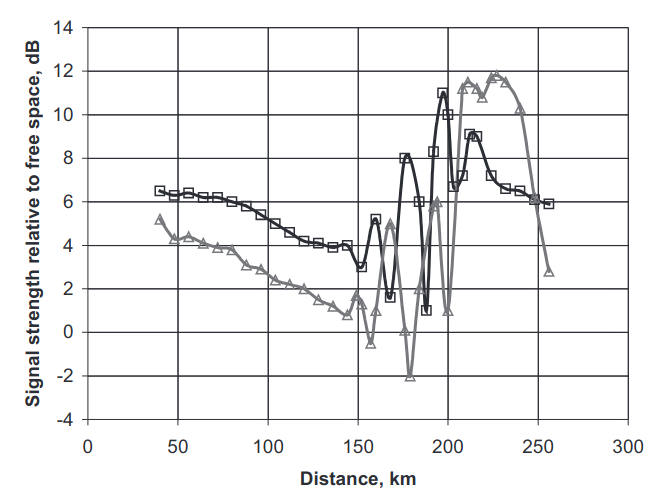
Attenuation factor — Fig. 5 The range dependence of the attenuation factor in a two-channel system: □, both antennas located inside the evaporation duct; △, antennas above the evaporation duct

At shorter distances the total field is a combination of the modes of the evaporation and elevated ducts with predominance of the evaporation duct. It also might be observed that at distances exceeding the first hop distance but still shorter than the second hop distance (in the above case with x > 200 km) the secondary excited field of the evaporation duct may provide a substantial contribution revealing a distinct change in the attenuation rate with distance and somewhat repeating the field at short range.

Figure 2 shows the ray trajectories for this situation. As observed, in the vicinity of the first hop the waves reflected from the elevated M-inversion provide a dominant contribution to the received field.

Author

Olga Nesvetailova

Freelancer

Literature

Jensen, N.O., Lenshow, D.H. An observational investigation on penetrative convection. J.Atmos.Sci., 1978, 35(10), 1924–1933.;
Monin, A.S., Yaglom, A.M. Statistical Fluid Mechanics, Vol.1, MIT Press, Cambridge, MA, 1971, p. 769.;
Gossard, E.E. Clear weather meteorological effects on propagations at frequencies above 1 GHz, Radio Sci., 1981,16(5), 589–608.;
Tatarskii, V.I. The Effects of Turbulent Atmo- sphere on Wave Propagation, IPST, Jerusalem, 1971.;
Gavrilov, A.S., Ponomareva, S.M. Turbulence Structure in the Ground Level Layer of the Atmosphere. Collected Data, Meteorology Series, No.1, Research Institute for Meteorological Information, Obninsk (in Russian), 1984.;
Kukushkin, A.V., Freilikher, V.D. and Fuks, I.M. Over-the-horizon propagation of UHF radio waves above the sea , Radiophys. Quantum Electron. (translated from Russian), Consultant Bureau, New York , RPQEAC 30 (7), 1987, 597–620.;

Footnotes