Exploring the Hartree-Fock Theory of the Evaporation Duct

Discover the essentials of Fock’s Theory and its application in the Hartree-Fock method for modeling evaporation ducts. This article delves into the principles of quantum mechanics, explaining how Fock’s approach enhances our understanding of atmospheric phenomena.

СодержаниеСвернуть

Basics of Fock’s Theory
Fock’s Theory of the Evaporation Duct

Learn about the significance of the Hartree-Fock theory in environmental science and its role in predicting evaporation duct behavior.

Basics of Fock’s Theory

In this section we briefly reproduce the basic results obtained by Fock for the vertical dipole in the case of normal refraction, in order to have a reference model for the further studies described in this category.

Following Fock, we introduce a non-dimensional distance and height ξ, h, respectively:

ξ = \frac{m x}{a}, h = \frac{k z}{m} E q . 1

where x = aθ and z = r–a, the same physical coordinates as defined in Parabolic Approximation to a Wave Equation in a Stratified Troposphere Filled with Turbulent Fluctuations of the Refractive Index“Parabolic Approximation to the Wave Propagation”. The relation between the Debye’s potential U and the slowly varying attenuation factor (envelope) V is given by:

U = \frac{e x p (j k a θ)}{\sqrt{a^{2} θ \sin θ}} V (ξ, h_{1}, h_{2}, q) E q . 2

where h₁ and h₂ are the non-dimensional heights of the receiver and transmitter, respectively, above the earth’s surface, ξ is the distance between them along the earth’s surface. A normalised impedance q is defined by:

q = \frac{j m}{\sqrt{η + 1}} . E q . 3

The attenuation factor V is given by a contour integral in a plane of complex parameter t:

V (ξ, h_{1}, h_{2}, q) = e x p (- j \frac{π}{4}) \sqrt{\frac{ξ}{π}} \int_{C} d t e x p (j ξ t) F (t, h_{1}, h_{2}, q) . E q . 4

The contour C comes from infinity in the second quadrant of the t-plane passing around and below all the poles of the integrand and then goes to infinity in the first quadrant of the t-plane. In the case of h2 > h1, the function F is given by:

F (t, h_{1}, h_{2}, q) = \frac{j}{2} w_{1} (t - h_{2}) [w_{2} (t - h_{1}) - \frac{w_{2}^{'} (t) - q w_{2} (t)}{w_{1}^{'} (t) - q w_{1} (t)} w_{1} (t - h_{1})] . E q . 5

In the case h₁ > h₂ we need to swap the h₁ and h₂ in the expression for F above. Three characteristic regions can be selected in the space of ξ, h₁, h₂ or, over the distance ξ, given fixed values of h₁, h₂. The first region is a line-of-sight region with

ξ < \sqrt{h_{1}} + \sqrt{h_{2}},

where the field is composed by superposition of the direct wave and the wave reflected from the earth’s surface. The second region is a shadow region at

ξ < \sqrt{h_{1}} + \sqrt{h_{2}},

where the electromagnetic field propagates only due to a diffraction mechanism and, finally, the third region is a transition region with

ξ \approx \sqrt{h_{1}} + \sqrt{h_{2}},

which separates the line-of-sight region from the shadow region. These regions are shown schematically in Figure 1. The transition region, also called a “shade cone”, is filled with dots in the figure.

Wave propagation — Fig. 1 Geometry of wave propagation

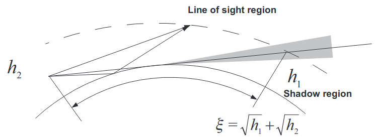
Fock obtained an asymptotical expansion of the integral (4) for all three regions. We reproduce his results for both the line-of-sight and the shadow regions.

In the shadow region the function F can be written in the following form:

F (t, h_{1}, h_{2}, q) = w_{1} (t - h_{2}) \frac{f (h_{1}, t)}{w_{1}^{'} (t) - q w_{1} (t)} E q . 6

where:

f (h_{1}, t) = [w_{1}^{'} (t) - q w_{1} (t)] ν (t - h_{1}) - [v^{'} (t) - q v (t)] w_{1} (t - h_{1}) . E q . 7

With h₁ = 0 the function f and its derivative have the values:

f (0, t) = 0, d f / d h_{1} = - q . E q . 8

The above equations can be obtained using the representation the Airy function w₁ via the Airy functions u and ν, see Airy Functions – Comprehensive Guide“In-Depth Exploration of Airy Functions and Their Applications”. From Eq. (8) one can find that if t = t_n is a root of the equation:

w_{1}^{'} (t) - q w_{1} (t) = 0, t = t_{1}, t_{2}, . . . E q . 9

the value of the function f is given by:

f (h_{1}, t_{s}) = f_{s} (h_{1}) = \frac{w_{1} (t_{s} - h_{1})}{w_{1} (t_{s})} E q . 10

and can be regarded as a height gain function of the mode with number s. In two limiting cases q = 0 and q = ∞ the roots ts can be estimated from asymptotic expressions valid for large s:

\begin{matrix} t_{s, q = 0} ≅ {[\frac{3 π}{2} (s - \frac{3}{4})]}^{2 / 3} e x p (j \frac{π}{3}), \\ t_{s, q = \infty} ≅ {[\frac{3 π}{2} (s - \frac{1}{4})]}^{2 / 3} e x p (j \frac{π}{3}), \end{matrix} E q . 11

and the first roots are as follows:

t_1,q=0=1,01879e^jπ/3;
t_1,q=∞=2,33811e^jπ/3.

The integral (4) can then be calculated as a sum of the residues in the poles of the integrand given by Eq. (9):

V (ξ, h_{1}, h_{2}, q) = e x p (j \frac{π}{4}) 2 \sqrt{π ξ} \sum_{s = 1}^{\infty} \frac{e^{j ξ t}}{1 - \frac{t_{s}}{q^{2}}} \frac{w_{1} (t_{s} - h_{1})}{w^{'} (t_{s})} \frac{w_{1} (t_{s} - h_{2})}{w^{'} (t_{s})} .

Equation (11) represents the series of the normal modes of the diffracted waves converging rapidly in a shadow region.

Consider the field in the line-of-sight interference region,

ξ < \sqrt{h_{1}} + \sqrt{h_{2}} .

In that region we have to obtain the reflection formula corresponding to the reflection from the spherical surface. The integral (4) can be represented by the sum of two terms:

V (ξ, h_{1}, h_{2}, q) = V_{d} - V_{r},

V_{d} = \frac{1}{2} e x p (j \frac{π}{4}) \sqrt{\frac{ξ}{π}} \int_{C} d t e x p (j ξ t) w_{1} (t - h_{2}) w_{2} (t - h_{1}), E q . 12

V_{r} = \frac{1}{2} e x p (j \frac{π}{4}) \sqrt{\frac{ξ}{π}} \int_{C} d t e x p (j ξ t) \frac{w_{2}^{'} (t) - q w_{2} (t)}{w_{1}^{'} (t) - q w_{1} (t)} w_{1} (t - h_{1}) w_{1} (t - h 2) . E q . 13

Assuming that the major contribution to integrals (12) and (13) comes from the interval of large and negative t we may use the asymptotic formulas for the Airy functions w₁ and w₂. Then for direct wave V_d we obtain:

V_{d} = \frac{1}{2} e x p (j \frac{π}{4}) \sqrt{\frac{ξ}{π}} \int_{C} d t \frac{e x p (j φ (t))}{{[(h_{1} - t) (h_{2} - t)]}^{1 / 4}} . E q . 14

The phase of the integrand φ(t) is given by:

φ (t) = ξ t + \frac{2}{3} {(h_{2} - t)}^{3 / 2} - \frac{2}{3} {(h_{1} - t)}^{3 / 2} .

The stationary value of t_s is determined from φ^′(t_s) = 0. The stationary value of the phase we denote as φ ≡ φ(t_s) and it is given by:

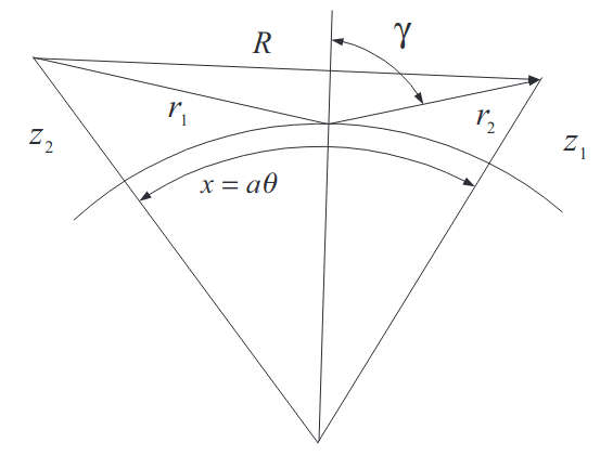
φ = \frac{{(h_{1} - h_{2})}^{2}}{4 ξ} + \frac{1}{2} ξ (h_{1} + h_{2}) - \frac{ξ^{3}}{12} . E q . 15

The value of φ has a simple geometric meaning of the difference between the phase of the direct wave along the distance R between the correspondents and the distance x = aθ along the earth’s surface, Figure 2:

Traces of the rays — Fig. 2 Ray traces in the line-of-sight region

φ = k (R - x) . E q . 16

Application of the stationary phase method to integral (14) leads to the following expression for the direct wave:

V_{d} = e x p (j φ) . E q . 17

Consider the term V_r. Using a similar asymptotic expression for the Airy function in the integrand we obtain:

V_{d} = \frac{1}{2} e x p (j \frac{π}{4}) \sqrt{\frac{ξ}{π}} \int_{C} d t \frac{e x p (j ψ (t))}{{[(h_{1} - t) (h_{2} - t)]}^{1 / 4} \frac{q - j \sqrt{- t}}{q + j \sqrt{- t}}} E q . 18

and:

ψ (t) = ξ t + \frac{2}{3} {(h_{2} - t)}^{3 / 2} + \frac{2}{3} {(h_{1} - t)}^{3 / 2} - \frac{4}{3} {(- t)}^{3 / 2} . E q . 19

The root of the equation

ψ^{'} (t) = 0

we define as t = –p², where p > 0. The stationary point in terms of p will be the root of the equation:

\sqrt{h_{1} + p^{2}} + \sqrt{h_{2} + p^{2}} = 2 p + x . E q . 20

The stationary value of the phase can then be defined in terms of the parameter p:

ψ = - 3 p^{2} ξ + 2 p (h_{1} + h_{2} - ξ^{2}) + ξ (h_{1} + h_{2}) - \frac{ξ^{3}}{3} . E q . 21

The application of the stationary phase method to Eq. (18) then results in the following expression for reflected wave:

V_{r} = \frac{q - j p}{q + j p} \sqrt{A} e x p (j ψ) E q . 22

with:

A = \frac{p x}{3 p x + x^{2} - h_{1} - h_{2}} . E q . 23

The formula (22) has the following geometric meaning. The parameter p is p = m cos (γ), where γ is an incidence angle as shown in Figure 2. The factor q-jp/q+jp is a Fresnel coefficient of reflection taken with the opposite sign. The parameter

\sqrt{A}

is a correction term accounting for divergence of the beam after reflection multiplied by a facto R/r₁, where r₁ is the distance along the ray from the source to the reflection point, Figure 2. The phase ψ can be written in a form similar to Eq. (16):

ψ = k (r_{1} + r_{2} - x) . E q . 24

Combining both terms in V we obtain the reflection formula:

V = e x p (j φ) - \frac{q - j p}{q + j p} \sqrt{A} e x p (j ψ) . E q . 25

The actual stationary value of p is given by:

p = \frac{1}{2 x} (h_{1} + h_{2} - \frac{1}{2} ξ^{2} + 4 ρ^{2} \sin^{2} (\frac{α}{3})) E q . 26

where:

ρ^{2} = \frac{1}{3} (ξ^{2} + 2 h_{1} + 2 h_{2}); \sin (α) = \frac{ξ (h_{1} - h_{2})}{ρ^{2}}; - \frac{π}{2} < α < \frac{π}{2} . E q . 27

The reflection formula (25) is valid for large enough p, practically it gives a good approximation for p > 2.

As will be discussed further, experimental results at frequencies above 1 GHz suggest little difference in the propagation of the vertically and horizontally polarised fields. As may be seen from the definition and values of m and η, parameter q is actually large for sea water at frequencies above 1 GHz, which suggests that, at least in the case of long range propagation, i. e. at distances beyond the opti- cal horizon, the impedance boundary conditions can be approximated by conditions for a vertically polarised field with q → ∞, practically suitable for both polarizations.

Fock’s Theory of the Evaporation Duct

In the case of the super-refraction associated with the evaporation duct the M-profile has one minimum at some height Z_s above the sea surface, called the height of the evaporation duct. Considering the case where q = ∞, the attenuation factor V(ξ, h₁, h₂, ∞) is given by Eq. (4) with the integrand F(t, h₁, h₂, ∞) given by:

F (t, h_{1}, h_{2}) = \frac{j}{2} f_{1} (t, h_{2}) [f_{2} (t, h_{1}) - \frac{f_{2} (0, t)}{f_{1} (0, t)} f_{1} (t, h_{1})] . E q . 28

and the height-gain functions f₁, f₂ are the solutions to the equation:

\frac{d^{2} f}{d h^{2}} + U (h) f = t f . E q . 29

The function U(h) is assumed to be an analytical function of its argument. We concentrate further on h and t where the equation U(h)-t = 0 has two roots: h = b₁ and h = b₂. For real t in the interval (U(H_s) < t ≤ U(0)), the above roots are also real.

Consider an asymptotical integration of Eq. (29) for height-gain functions which is valid for all values h and t, including t = U(H_s), i. e. the point of the minimum of the U-profile. The asymptotical solution in this case should be built upon an “etalon” equation, which behaves similarly to Eq. (29), i. e. has a single minimum, and, on the other hand, has a known analytical solution. The “etalon” equation can be expressed in the form of an equation for functions of a parabolic cylinder:

\frac{d^{2} g}{d ς^{2}} + [\frac{1}{4} ς^{2} + ν] g = 0 . E q . 30

The relation between Eqs. (30) and (29) is established by a transformation of h into ς in a form which ensures that two conditions are met:

The parameter U(h)-t in Eq. (29) has the same roots as 1/4 ς²+ν, and;
With large values of the above parameters, either Eq. (29) or Eq. (30) results in the same asymptotic expression for their respective solutions f and g.

Such conditions are satisfied with the following substitution:

\int_{b_{1}}^{h} \sqrt{U (h) - t} d h = \frac{1}{2} \int_{- 2 j \sqrt{ν}}^{ς} \sqrt{ς^{2} + 4 ν} d ς E q . 31

with parameter ν bounded by following equation:

\int_{b_{1}}^{b_{2}} \sqrt{U (h) - t} d h = \frac{1}{2} \int_{- 2 j \sqrt{ν}}^{2 j \sqrt{ν}} \sqrt{ς^{2} + 4 ν} d ς . E q . 32

The value integral in Eq. (30) results in the relationship between roots b₁, b₂, and ν:

j π ν = \int_{b_{1}}^{b_{2}} \sqrt{U (h) - t} d h .

Expanding the right-hand side of Eq. (32) into a Taylor series in the vicinity of the minimum of U(h) we obtain ν as a holomorphic function of t:

ν = \frac{U (H_{s}) - t}{\sqrt{2 U^{''} (H_{s})}} + . . . E q . 33

Since U^′′(H_S) > 0, we can read formula (32) in the following way: ν > 0 when t < U(H_s) and ν < 0 when t > U(H_s); with U(H_s) < t < U(0) we then have:

ν = - \frac{1}{π} \int_{b_{1}}^{b_{2}} \sqrt{t - U (h)} d h . E q . 34

Then, introducing the notations for the phase terms:

S = \int_{0}^{h} \sqrt{U (h) - t} d h, S_{0} = \frac{1}{2} \int_{0}^{b_{1}} \sqrt{U (h) - t} d h + \frac{1}{2} \int_{0}^{b_{2}} \sqrt{U (h) - t} d h, E q . 35

the substitution (31), which in fact defines the relation between h and ς, can be expressed in the form:

S (h) - S_{0} = \frac{1}{2} \int_{- 2 j \sqrt{ν}}^{ς} \sqrt{ς^{2} + 4 ν} d ς = \frac{1}{4} ς \sqrt{ς^{2} + 4 ν} + ν \ln (ς + \sqrt{ς^{2} + 4 ν}) - \frac{ν}{2} \ln (4 ν) . E q . 36

The respective solutions of Eqs. (29) and (30) are related as follows:

f = \sqrt{\frac{d h}{d ς}} g E q . 37

where function g, the solution to Eq. (30), can be expressed via a function of a parabolic cylinder D_n(z), given by the series:

D_{n} (z) = \frac{2^{- \frac{n}{2} - 1}}{Γ (- n)} e^{- \frac{z^{2}}{4}} \sum_{m = 0}^{\infty} \frac{Γ (\frac{m - n}{2})}{Γ (m + 1)} 2^{\frac{m}{2}} {(- z)}^{m} . E q . 38

Function D_n(z) will obey Eq. (30) when n = jν-1/2 and z = ςe^jπ/4. The appropriate solutions to Eq. (29) are then given by:

\begin{matrix} f_{1} (h, t) = c_{1} (ν) \sqrt{2 \frac{d h}{d ς}} g_{1} (ς), \\ f_{2} (h, t) = c_{2} (ν) \sqrt{2 \frac{d h}{d ς}} g_{2} (ς) \end{matrix} E q . 39

and:

\begin{matrix} g_{1} (ς) = D_{j ν - 1 / 2} (ς e^{- j π / 4}), \\ g_{2} (ς) = D_{- j ν - 1 / 2} (ς e^{j π / 4}), \end{matrix} E q . 40

\begin{matrix} c_{1} (ν) = e x p [- \frac{π ν}{4} + j \frac{π}{8} + j (\frac{1}{2} ν - \frac{1}{2} ν \ln (ν) - S_{0})], \\ c_{2} (ν) = c_{1} {(ν)}^{*} = e x p [- \frac{π ν}{4} - j \frac{π}{8} - j (\frac{1}{2} ν - \frac{1}{2} ν \ln (ν) - S_{0})] . \end{matrix} E q . 41

The coefficients c₁(ν) and c₂(ν) are defined by Eq. (42) with the aim being to obtain a correct asymptotic expression for f₁ (h, t), f₂ (h, t) with large values of the argument h and holomorphic functions (40) in the vicinity of ν = 0.

With large positive ς, that corresponds to large heights h, well above H_s, the height gain functions take the following asymptotic forms:

\begin{matrix} f_{1} (h, t) = \frac{e^{π / 4}}{\sqrt[4]{U (h) - t}} e x p (j (S - 2 S_{0})), \\ f_{2} (h, t) = \frac{e^{- j π / 4}}{\sqrt[4]{U (h) - t}} e x p (- j (S - 2 S_{0})) . \end{matrix} E q . 42

Inside the evaporation duct and, strictly speaking, far below the inversion height H_s when ς is large and negative, the asymptotic representations for the height-gain functions take the form:

\begin{matrix} f_{1} (h, t) = χ_{1} (ν) \frac{e^{j π / 4}}{\sqrt[4]{U (h) - t}} e x p (j (S - 2 S_{0})) + e^{- π ν} \frac{e^{- j π / 4}}{\sqrt[4]{U (h) - t}} e x p (- j S), \\ f_{2} (h, t) = χ_{2} (ν) \frac{e^{- j π / 4}}{\sqrt[4]{U (h) - t}} e x p (- j (S - 2 S_{0})) + e^{- π ν} \frac{e^{j π / 4}}{\sqrt[4]{U (h) - t}} e x p (j S) \end{matrix} E q . 43

where:

\begin{matrix} χ_{1} (ν) = \frac{\sqrt{2 π}}{Γ (\frac{1}{2} - j v)} e x p [- \frac{π ν}{2} + j (ν - ν \ln (ν))], \\ χ_{2} (ν) = \frac{\sqrt{2 π}}{Γ (\frac{1}{2} + j v)} e x p [- \frac{π ν}{2} - j (ν - ν \ln (ν))] . \end{matrix} E q . 44

The asymptotic representation of the integrand (28) is then given by:

F (t, h_{1}, h_{2}) = \frac{j}{2} \frac{1}{\sqrt[4]{U (h_{1}) - t} \cdot \sqrt[4]{U (h_{2}) - t}} \cdot \frac{[e^{j S (h_{1})} - Λ e^{- j S (h)}] \cdot [e^{- j S (h_{2})} - e^{j S (h_{2})}]}{1 - Λ} E q . 45

with H_s > h₁ > h₂ , where:

Λ = j \frac{e^{- π ν + 2 j S_{0}}}{χ_{1} (ν)} . E q . 46

The poles in the integral (4) with the integrand in the form (45) will be given by the roots of the characteristic equation:

1 - Λ = 0 . E q . 47

In many practical cases the evaporation duct parameters are such that the values of parameter ς are of the order of 1, or even less, in Eqs. (45) and (47). Therefore, some doubts can be raised as to the validity of the asymptotic formulas (46) and (47) in this case. Fock calculated the propagation constants given by Eq. (45) and the exact equation:

g_{1} (0, t) = 0 . E q . 48

expressed via functions of a parabolic cylinder. A sample of the calculations of propagation constants for the hyperbolic profile:

U (h) = \frac{(h - H_{s})}{h + h_{l}}, E q . 49

where h_l is a parameter, is presented in table.

Comparison of the calculated propagation constants using the asymptotic Eq. (47) and the exact formula (48)
H_s+h_l	Asymptotic t₁	Exact t₁
23,11	-0,085+j0,466	-0,107+j0,443
25,24	-0,148+j0,262	-0,158+j0,269
48,07	-0,104+j0,224	-0,113+j0,227

As observed, the agreement between the asymptotic formulas and the exact solution is satisfactory, especially with regard to the imaginary part of the propagation constants, Im(t_n). The relation between the attenuation rate of the nth mode, γn, and Im(t_n) is given by:

γ_{n} = 0, 434 \frac{k}{m^{2}} Im (t_{n}), d B / k m . E q . 50

Consider Eq. (47) for trapped modes which have a small imaginary component of the propagation constant tn and are in the interval: U(H_s) ≤ Re t_n < U(0). The respective values of parameter v are negative. For v < 0 we define ln(ν) = ln(-ν)+jπ and from Eq. (35) we obtain:

S_{0} = \int_{0}^{b_{1}} \sqrt{U (h) - t} d h - j \frac{π}{2} ν \equiv S_{1} - j \frac{π}{2} ν . E q . 51

Equation (47) then takes the form:

j e^{2 j S_{1}} = χ (ν) ≅ 1 . E q . 52

For large negative ν, χ(ν) → 1, and we obtain:

S_{1} \equiv \int_{0}^{b_{1}} \sqrt{U (h) - t} d h = (m - \frac{1}{4}) π, m = 1, 2, . . . E q . 53

For either large positive ν or complex ν with positive Re ν, it follows that Re t < U(H_s). In this case the phase S₁ can be defined as:

S_{1} = S_{0} + j \frac{π}{2} ν E q . 54

and Eq. (47) will again be truncated to Eq. (53).

A basic conclusion followed from the study of Eq. (47) and its truncated form (53) (performed by Fock) is that the attenuation rate of the field in the evaporation duct is affected not only by the height Z_s and the M-deficit of the evaporation duct but also by a curvature of the M-profile at the level of inversion height Z_s. The attenuation rate γ_m of the mth mode from Eq. (53) can be estimated as follows:

γ_{m} = 2 π (m - \frac{1}{4}) 10^{- 3} \frac{Z_{s} M^{''} (Z_{s})}{β \sqrt{2 (M (0) - M (Z_{s}))}} Θ = \frac{2 π}{λ_{m}} 10^{- 6} Z_{s}^{2} M^{''} (Z_{s}) Θ E q . 55

where:

Θ = \frac{λ_{m}}{λ} Im t_{m}; E q . 56

λ_{m} = \frac{β 10^{3} Z_{s}}{m - 1 / 4} \sqrt{2 (M (0) - M (Z_{s}))}

is a critical wavelength of the mth mode trapped in the evaporation duct formed by a given M-profile, λ is the wavelength of the radiated field. The parameter β is introduced by:

β = \int_{0}^{1} q (z) d z; q (0) = 4; q (1) = 0; E q . 57

q (\frac{z}{Z_{s}}) = 4 \frac{M (z) - M (Z_{s})}{M (0) - M (Z_{s})} . E q . 58

For most M-profiles the value of β is close to 1.

Author

Olga Nesvetailova

Freelancer

Literature

Fock, V.A. Electromagnetic Diffraction and Propagation Problems, Pergamon Press, Oxford, 1965.
Fock, V.A. Distribution of currents excited by a plane wave on the surface of conductor, J. Exp. Theor. Phys., (Nauka), 1945, 15 (12), 693–702.
Leontovitch, M.A. Method of solution to the problems of em wave propagation over the boundary surface, Izv. Acad. Nauk, Ser. Fiz., 1944, 8 (1), 16–22.
Leontovitch, M.A., Fock, V.A. Solution to a problem of em wave propagation over the Earth’s surface using the method of parabolic equation, J. Exp.Theor. Phys., (Nauka), 1946, 16 (7), 557–573.
Fock, V.A. Theory of wave propagation in a non-uniform atmosphere for elevated source, Izv. Acad. Nauk, Ser. Fiz., 1960, 14 (1), 70–94.
Krasnushkin, A.E. The expansion over normal waves in a spherically-stratified medium, Dokl. Acad. Nauk SSSR, 1969, 185 (6), 1262–1265.
Kravtsov, Yu.A., Orlov, Yu.I., Geometric Optics of Non-uniform Media, Nauka, Moscow, 1980, 340 pp.
Rotheram, S. Radiowave propagation in the evaporation duct, The Marconi Rev., 1974, 67 (12), 18–40.
Booker, H.G., Walkinshaw W. The mode theory of tropospheric refraction and its relation to waveguides and diffraction, in Meteorological Factors in Radiowave Propagation, The Royal Society, London, 1946, pp. 80–127.
Andrianov, V.A. Diffraction of UHF in a bilinear model of the troposphere over the Earth’s surface, Radiophys. Quantum Electron., 1977, 22 (2), 212–222.
Wait, J.R. Electromagnetic Waves in Stratified Media, Pergamon Press, Oxford, 1962, 372 pp.
Hitney, H.V., Pappert, R.A., Hattan, C.P. Evaporation duct influences on beyond-the-horizon high altitude signals, Radio Sci., 1978, 13 (4), 669–675.
Chang, H.T. The effect of tropospheric layer structures on long-range VHF radio propagation, IEEE Trans. Antennas and Propagation, 1971, 19 (6), 751–756.
Wait, J.R., Spies, K.P. Internal guiding of microwave by an elvated tropospheric layer, Radio Sci., 1964, 4 (4), 319–326.
Gerks, I.H. Propagation in a super-refractive troposphere with a trapping surface layer, Radio Sci., 1969, 4 (5), 413–417.

Footnotes