Understanding Parabolic Approximation in Wave Propagation: Analytical Methods and Applications

Discover the intricacies of wave propagation through stratified and random media with our in-depth analysis of parabolic approximation methods. This article covers the application of the wave equation in turbulent tropospheres, highlighting the impact of refractive index fluctuations.

Learn about the Green function for parabolic equations in stratified environments and enhance your knowledge of wave behavior in complex settings.

Analytical Methods in the Problems of Wave Propagation in a Stratified and Random Medium

The analogy between the non-stationary problem of quantum mechanics and the parabolic approximation in a problem wave propagation was likely first explored by Fock. It is well known that the methods of classic wave theory were utilised in quantum mechanics in the early stages of its development. At present, the situation is rather the reverse, and the mathematical methods of quantum mechanics have become widely adopted in the latest developments of wave theory.

The asymptotic solution to the problem of the diffraction of a plane monochromatic wave over a sphere of large radius, compared with the wavelength of radiation, was obtained by Fock in 1945. In obtaining this solution, he developed an asymptotic theory of diffraction on the basis of Leontovich’s boundary conditions and the concept of the “local” field. The approach utilised several large parameters involved in problem formulation, such as |η| ≫ 1, m = (kα/2)^1/3 ≫ 1, η = ε_g+j4πσω, ε_g, σ, the dielectric permittivity and conductivity of the earth, respectively, ω is the cyclic frequency of the radiated wave, k = 2p/λ is a wavenumber, λ is a wavelength, α is the radius of the earth’s sphere. The same results were obtained by Fock later by means of the parabolic approximation to the wave equation which is based on significantly different parameters, with m ≫ 1, and the characteristic scales of the wave oscillations in two different directions: along the earth’s surface and normal to it. With regards to radio wave propagation at a frequency above 1 GHz the important development was a solution of the parabolic equation for the stratified troposphere, where the refractive index depends solely on the height above the ground surface.

The analysis of the wave field at low altitudes z, which are small compared with the radius of the earth’s curvature α, is convenient to perform by means of the introduction of the modified refractivity:

The solution obtained is suitable for the very general case of the dependence n(z) and impedance boundary conditions at the earth’s surface. The solution is represented by a contour integral which in the shadow region is calculated by a sum over residues in the poles of the integrand, i. e. a series of normal waves. In the line-of-sight (LOS) region the contour integral is commonly calculated using stationary phase methods similar to a geometric optic approximation. Further study of the wave propagation in a stratified tropo- sphere was dedicated to the development of the effective methods of the field representation for various height profiles of the refractivity and combinations of the relative location of the transmitting and receiving antennae. An alternative analytical method to the solution of wave propagation in stratified medium, the method of “invariant submergence”, was developed by Klatskin. Using that method, a boundary problem, which is, in fact, a problem of diffraction, can be transformed into a problem of evolution. A significant advantage of this method is its inherent capability to study the wave propagation through random media, and the method is especially effective when applied to a randomly stratified medium.

Together with a ducting mechanism, the wave scattering on random inhomogeneities of the refractive index plays a significant role in the study of radio wave propa- gation in the atmospheric boundary layer at frequencies above 1 GHz. The straight-forward application of either the contour integral or normal mode series to a problem of wave propagation in a random troposphere will face significant difficulties. The major problem will be related to the divergence of the matrix elements of the normal wave transformation due to a scattering on random fluctuations in the refractive index. The deployment of the method of “invariant submergence” also does not lead to an analytical solution to the problem though numerical calculation is possible.

In this category we use the representation of the Green function in the form of an expansion over the eigen functions of a continuous spectrum which allows one to avoid the above mentioned difficulties of divergence of matrix elements and then to separate the matrix coefficients with a “nearly discrete” and continuum spectrum with normalised height gain functions. This approach led to some advances in solving several problems, in particular, the problem of wave propagation in a tropospheric duct filled with random irregularities of the refractive index in addition to a regular supper-refractive gradient of the refractivity. The disadvantage of the method is that the separation of the discrete spectrum of eigen functions is performed in the “unperturbed”, i. e. regular, part of the Schrödinger operator and, therefore, the spectrum of eigen functions is left unchanged by the random component of the potential term. The study of the spectrum of Schrödinger’s equation with random potential is a complex problem by itself and most advances so far have been achieved in the one-dimensional problem.

The theory of wave scattering in a random medium has been developed during the last decades. The most significant progress has been achieved in the solution to the problems of wave propagation in either a random but unbound medium or a uniform medium with a random boundary interface. In the solution of these problems a statistical approach is commonly used. This approach is targeted at obtaining the statistical characteristics of the scattered field:

• probability function or,
• statistical moments of the field.

Among them the first two moments: average field (coherent component) and either coherence function or field intensity, are of significant interest in many practical applications. There are three known methods of obtaining the closed equations for the field moments: Feynman diagrams, local perturbation and the Markov process approximation.

The study of a coherent component can be done using the modified perturbation theory, a similar result is obtained from the diagram methods. The advances in the solution of the higher order moments of the field have been obtained after application of the parabolic approximation to the wave equation. Neglecting back scattering in the parabolic approximation allows one to employ the concept of the Markov process and all the following analogies from the statistical theory of Markov processes.

The advantage of the functional approach, is that the formal solution to the problem is written via quadrature. The moment of the field of any order can, in principle, be obtained by averaging the respective dynamic solution which is described by a multiple functional integral in the space of the virtual trajectories. The solutions to the first two moments of the field obtained from both the method of closed equations for the moments and the method of the path integral provide exactly the same result, under conditions of the Markov process approximation. The study of the field moments of order higher than two is easier with the use of the path integral, since this approach does not formally require a solution of the equations for the field moments. In fact, this advantage became apparent in the calculation of the moments of the intensity (signal strength), which are not described by a closed equation.

The current limitations of the path integral method could be rather associated with the still limited mathematical methods of analytical calculation of the trajectory integrals, despite the serious studies in that area.

Finally, we comment on studies concerning scattering on a rough sea surface. The basic conclusion is that, until now, there is no adequate theory that takes into account the combined effect of refraction, diffraction and scattering on random inhomegeneities of the refractive index in the volume of the tropospheric layer as well as scattering on a rough sea surface. The impact from a rough surface cannot be regarded as negligible in the general case, at least from a theoretical point of view. Known attempts are limited to the deterministic model of the sea surface or a semi-empirical approach in treating the scattering on the sea surface in the Kirchhoff approximation that is applicable to the coherent component of the scattered field. While the theory of wave scattering on a random surface is an established science by itself, the studies known to the author were concerned with scattering theory on a random surface while treating the propagation media in a very simplistic way, basically, as deterministic and uniform.

In applying the scattering theory to a ducting mechanism, the approach should eventually be modified in order to take into account the multiple effects of refraction, diffraction and scattering. As discussed in Atmospheric Boundary Layer and Basics of the Propagation Mechanisms“Atmospheric Boundary Layer and Key Propagation Mechanisms”, the sea waves could be responsible for the modulation of the turbulence spectrum in the near-surface layer, where the major action of radio propagation takes place. On the other hand, all previous advances in theory have been driven by some unresolved problems in experiments on the radio wave propagation phenomenon. So far, the currently available radio coverage prediction system is reported to be in reasonably good agreement with the results of existing models, at least for measured signal strength.

Parabolic Approximation to a Wave Equation in a Stratified Troposphere Filled with Turbulent Fluctuations of the Refractive Index

Let us consider the vertical electric dipole in a spherical coordinate system (r, ϑ, ϕ) with the spherical axis coming through the dipole. Assume that the dielectric permeability ε is a function of the radius only, e. g. ε = ε(r). The classical solution to the electromagnetic field can be derived by introduction of Debye’s potentials U and V.

The field components are given by the following equations:

We assume the field to be a harmonic function of time – exp (-jωt), ω is a cyclic frequency of the electromagnetic radiation, k = ω/c is a wave number, and c is the speed of light. The notation Δ* represents a Laplace operator on a sphere:

The Maxwell equations:

will be satisfied if potentials U and V obey the following equations:

The approximate Leontovitch’s boundary conditions for U and V have the form:

with r = α, where a is the earth’s radius.

where $\partial \epsilon \left(\overrightarrow{r}\right)$

is a random component present in each realisation of

$\epsilon \left(\overrightarrow{r}\right)$

, and

Assume also that |δε/ε| ≪ 1. The angular brackets here and below mean averaging over the statistical ensemble of the fluctuations δε.

Let us assume that, the relationships between field components

$\overrightarrow{E}, \overrightarrow{H}$

and potentials U, V are still given by Eqs. (1) and (2). Strictly speaking, the Maxwell equations (4) cannot be satisfied for an arbitrary function

$\delta \epsilon \left(\overrightarrow{r}\right)$

, and one can seek approximation to Eq. (4) where the divergent terms are small.

Introduce vector

$\overrightarrow{x}=\left\{\alpha \vartheta , \varphi r \sin \vartheta \right\}.$

The divergent terms in Eq. (4) will be small when:

$\left|\frac{\partial \epsilon }{\partial x_i}\right|\ll k Eq. 9$

where x_i is any of component of the vector

$\overrightarrow{x}.$

When the inequality (2.12) holds, the potentials U and V are governed by Atmospheric Boundary Layer and Basics of the Propagation MechanismsEq. 8), Atmospheric Boundary Layer and Basics of the Propagation MechanismsEq. 9 where

$\epsilon ={\epsilon }_0\left(r\right)+\delta \epsilon \left(\overrightarrow{r}\right).$

Let us examine the vertically polarised field for which V = 0, U ≠ 0. For high frequencies when kα >> 1, we can select a “dedicated” direction of wave propagation x = αϑ aligned with the direction along the arc of the earth’s radius. With kα >> 1, the radial component of the electric field E_r is related to the potential U via: E_r ≈ -kα² U.

Introduce a new function:

$U_1=\epsilon rU Eq. 10$

which is governed by the equation:

$\frac{\partial }{\partial r}\left(\frac{1}{\epsilon }\frac{\partial U_1}{\partial r}\right)+\frac{1}{\epsilon r^2}\left[\frac{{\partial }^2{U}_1}{\partial {\vartheta }^2}–\frac{\partial U_1}{\partial \vartheta }\left(\frac{2}{\epsilon }\frac{\partial \epsilon }{\partial \vartheta }–\frac{\cos \vartheta }{\cos \vartheta }\right)+U_1\left(\frac{1}{{\epsilon }^2}{\left(\frac{\partial \epsilon }{\partial \omega }\right)}^2–\frac{1}{\epsilon }\frac{{\partial }^2\epsilon }{\partial {\vartheta }^2}–\frac{\cos \vartheta }{\epsilon \sin \vartheta }\frac{\partial \epsilon }{\partial \vartheta }\right)\right]+\frac{1}{\epsilon r^2 \sin \vartheta }\left[\frac{{\partial }^2{U}_1}{\partial {\phi }^2}–\frac{2}{\epsilon }\frac{\partial U_1}{\partial \phi }\frac{\partial \epsilon }{\partial \varphi }–\frac{U_1}{{\epsilon }^2}\left(\frac{{\partial }^2\epsilon }{\partial {\phi }^2}–\frac{2}{\epsilon }{\left(\frac{\partial \epsilon }{\partial \phi }\right)}^2\right)\right]+k^2{U}_1=0 Eq. 11$

and obeys the boundary condition:

$\frac{\partial \left(U_1\right)}{\partial r}=–jk\frac{U_1}{\sqrt{\eta +1}}, \mathrm{with} r=\alpha . Eq. 12$

Let us isolate the slow varying complex amplitude W₁ in the wave field by:

$U_1=W_1{e}^{jk\alpha \vartheta } Eq. 13$

and introduce coordinate γ = (r sin ϑ)φ. The amplitude W₁ is then given by equation:

$\frac{{\partial }^2{W}_1}{\partial r^2}+\frac{2jk}{r}\frac{\partial W_1}{\partial \vartheta }+\frac{{\partial }^2{W}_1}{\partial {\gamma }^2}+\left(k^2\epsilon –k^2\frac{{\alpha }^2}{r^2}\right)W_1=\frac{\partial \epsilon }{\partial r}\frac{\partial W_1}{\partial r}–\frac{1}{r^2}\frac{{\partial }^2{W}_1}{\partial {\vartheta }^2}+j\frac{k}{r}{W}_1\left(\frac{2}{\epsilon }\frac{\partial \epsilon }{\partial \vartheta }–\frac{\cos \vartheta }{\sin \vartheta }\right)+\frac{W_1}{r^2}\left(\frac{1}{{\epsilon }^2}{\left(\frac{\partial \epsilon }{\partial \vartheta }\right)}^2–\frac{1}{\epsilon }\frac{{\partial }^2\epsilon }{\partial {\vartheta }^2}–\frac{\cos \vartheta }{\epsilon \sin \vartheta }\frac{\partial \epsilon }{\partial \vartheta }\right)+\frac{1}{r^2}\left[\frac{2}{\epsilon }\frac{\partial W_1}{\partial \gamma }\frac{\partial \epsilon }{\partial \gamma }–\frac{W_1}{\epsilon }\left(\frac{{\partial }^2\epsilon }{\partial {\gamma }^2}–\frac{2}{\epsilon }{\left(\frac{\partial \epsilon }{\partial \gamma }\right)}^2\right)\right] Eq. 14$

at the right-hand side of which we have a correction term. Using qualitative arguments, it can be shown that in the case of a stratified medium ε = ε(r) the terms on the left have an order of magnitude of k²W₁/m² while on the right the terms containing derivatives are of the order of k²W₁/m⁴. The right-hand side terms containing sin ϑ in the denominator will also be small if the following inequality holds:

$x\gg \frac{\alpha }{m}. Eq. 15$

The problem now is to evaluate the terms in the right-hand side of Eq. (14) for the case of random

$\delta \epsilon \left(\overrightarrow{r}\right)$

caused by turbulence. Let us introduce coordinate z = r-α. The characteristic scales L of variations in W₁ over x, y, z can be estimated as follows:

$L_x~\frac{\alpha }{m}, L_{\gamma }~\sqrt{\lambda x}, L_z~\frac{m}{k}. Eq. 16$

respectively. Having compared the terms in the left- and right-hand sides of Eq. (14) we obtain the inequalities:

${\left(\frac{\partial \epsilon }{\partial x}\right)}^2\ll \frac{m^2}{{\alpha }^2}, {\left(\frac{\partial \epsilon }{\partial \gamma }\right)}^2\ll \frac{1}{\lambda x}, {\left(\frac{\partial \epsilon }{\partial z}\right)}^2\ll \frac{k^2}{m^2} Eq. 17$

which, being satisfied, allow one to treat the terms in the right-hand side of Eq. (14) as negligible. Therefore, with fulfilment of inequalities (17) the right-hand side of Eq. (14) can be replaced with zero.

The inequalities (17) put limitations chiefly on the intensity of small-scale fluctuations

$\delta \epsilon \left(\overrightarrow{r}\right)$

. We can assume that the fluctuations in dielectric permittivity

$\delta \epsilon \left(\overrightarrow{r}\right)$

are locally uniform and isotropic. Let us introduce a spatial spectrum Φ_ε of fluctuations

$\delta \epsilon \left(\overrightarrow{r}\right)$

by the equation:

${\Phi }_{\epsilon }\left(\overrightarrow{\kappa }\right)=\frac{1}{16{\mathrm{\pi }}^3}\int d^3\overrightarrow{\rho }·\mathrm{grad}<{\left[\delta \epsilon \left(\overrightarrow{r}+\overrightarrow{\rho }\right)–\delta \epsilon \left(\overrightarrow{r}\right)\right]}^{\mathrm{2}}>\frac{\overrightarrow{\kappa } \sin \left(\overrightarrow{\mathit{k}}\overrightarrow{\mathit{\rho }}\right)}{\kappa } Eq. 18$

where

$\overrightarrow{\kappa }=\left\{{\kappa }_x, {\kappa }_{\gamma }, {\kappa }_z\right\}$

is the wave vector of the fluctuations in the dielectric permittivity,

$\kappa =\left|\overrightarrow{\kappa }\right|.$

We can evaluate the gradients in

$\delta \epsilon \left(\overrightarrow{r}\right)$

by:

where x_n is any of the coordinates x, y, z. For the spatial spectrum of fluctuations

$\delta \epsilon \left(\overrightarrow{r}\right)$

we can use the formula related to the equilibrium interval of the locally-isotropic turbulence:

${\Phi }_{\epsilon }\left(\overrightarrow{\kappa }\right)=0,033 C_{\epsilon }^2{\kappa }^{–11/3}\exp \left(–\frac{{\kappa }^2}{{\kappa }_m^2}\right) Eq. 20$

where c_z is a structure constant, κ_m = 5,92/l₀, l₀ is an internal scale of turbulence. Substituting Eq. (20) into Eq. (17) we obtain:

$0,033 C_{\epsilon }^2 {\kappa }_m^{4/3}\ll \frac{k}{x},\frac{k^2}{m^2},\frac{m^2}{{\alpha }^2}. Eq. 21$

Assuming reasonably short distances and high frequencies of radiation, e. g. m ≫ 1 and x ≤ 10³km, we can see that the major impact comes from variations of the z-coordinate, and the inequality (22) thus reduces to:

$0,033 C_{\epsilon }^2\mathrm{\pi }{\left(\frac{\alpha }{2}\right)}^{2/3}{\left(\frac{\lambda }{l_0}\right)}^{4/3} \ll 1. Eq. 22$

Here we took into account that k/m = k^2/3 (α/2)^1/3. Estimating the parameters

$C_{\epsilon }^2={10}^{–14}c{m}^{–2/3}, \alpha =8 500 km$

, we observe that the coefficient with (λ/l₀)^4/3 has an order of 10^–9.

Now we can conclude that with fulfilment of inequalities (15), (22) and z/α ≪ 1, the complex amplitude

$W_1\left(\overrightarrow{r}\right)$

obeys the approximate equation:

$j2k\frac{\partial W_1}{\partial x}+\frac{{\partial }^2{W}_1}{\partial {\gamma }^2}–\frac{{\partial }^2{W}_1}{\partial z^2}+k^2\left({\epsilon }_m\left(z\right)–1+\delta \epsilon \left(\overrightarrow{r}\right)\right) W_1=0 Eq. 23$

and boundary condition:

$\frac{\partial W_1}{\partial z}=–jk\frac{W_1}{\sqrt{\eta +1}} \mathrm{with} z=0 Eq. 24$

The potential U is given by:

$U\left(\overrightarrow{r}\right)=\frac{e^{jka\vartheta }}{\epsilon r}{W}_1\left(\overrightarrow{r}\right). Eq. 25$

The next step is to figure out the correct representation of the field amplitude W₁ at small distances from the source in order to obtain an initial condition. In particular, at the distance where the curvature of the earth can be neglected as well as the ray’s refraction we have to obtain a reflection formula in the parabolic approximation. Introducing the coordinates of the source:

• x = 0;
• γ = γ₀;
• z = z₀;
• and assuming that η ≫ 1 the reflection formula will be satisfied when:

$W_1\left(x, \overrightarrow{\rho }\right)=2\frac{\epsilon \left(x, \overrightarrow{\rho }\right)}{x}\alpha exp \left\{j\frac{k}{x}{\left(\overrightarrow{\rho }–{\overrightarrow{\rho }}_0\right)}^2\right\} Eq. 26$

where

$\stackrel{\rightharpoonup }{\rho }=\left\{\gamma , z\right\}, {\stackrel{\rightharpoonup }{\rho }}_0=\left\{{\gamma }_0, z_0\right\}.$

Taking into account the relationship:

$lim{|}_{x\to x^{\prime }}\frac{k}{2\mathrm{\pi }\left(x–x^{\prime }\right)}exp\left\{j\frac{k}{\left(x–x^{\prime }\right)}{\left(\overrightarrow{\rho }–{\overrightarrow{\rho }}^{\prime }\right)}^2\right\}=\partial \left(\overrightarrow{\rho }–{\overrightarrow{\rho }}^{\prime }\right)$

where

$\delta \left(\overrightarrow{\rho }\right)$

is a Dirac’s delta-function defined by:

$\delta \left(\overrightarrow{\rho }\right)=\frac{1}{4{\mathrm{\pi }}^2}\int d^2\overrightarrow{\kappa } exp \left(j\overrightarrow{\kappa }\overrightarrow{\rho }\right), Eq. 27$

we make a transition in Eq. (27) with x → 0 and obtain an expression for singularity at the source:

$lim{|}_{x\to 0}{W}_1\left(x, \overrightarrow{\rho }\right)=4\mathrm{\pi }j\epsilon \left(0, {\overrightarrow{\rho }}_0\right)\frac{\alpha }{k}\delta \left(\overrightarrow{\rho }–{\overrightarrow{\rho }}_0\right). Eq. 28$

Equation (27) shall take place in a line-of-sight region, i. e. with

$x\ll \sqrt{2\alpha z_0}.$

Taking into account that the inequality (16) is to hold as well, we obtain the limitations at the height of the source z₀ under which the expression (29) is valid:

$z_0\gg \alpha /m^2. Eq. 29$

It should be noted that in the case of very small heights of the source, another approach can be used and the solution to Eq. (24) should be tailored with the solution of Veil-Van-der-Paul at small distances x.

In conclusion, one should note that there is some ambiguity with the definition of the complex amplitude via Debye’s potential U. Indeed, equations similar to Eq. (24) can be obtained for the other functions W₂ and W₃ defined by the following expressions:

$\begin{array}{c}{W}_2=\epsilon r{\sqrt{\sin \vartheta ·e}}^{–jk\alpha \vartheta }U,\\ W_3=\epsilon r \sin {\vartheta }^{–jk\alpha \vartheta }U.\end{array} Eq. 30$

The area of applicability of the parabolic approximation for W₃ is defined by the same set of inequalities (16), (22) while for W₃ the inequality (16) can be replaced by a less stringent one:

$x\gg m/k. Eq. 31$

Let us summarize the major steps undertaken in this section:

• The components of the electromagnetic field
  $\overrightarrow{E}$
  and
  $\overrightarrow{H}$
  can be represented via Debye’s potentials U and V. Even in the presence of a random turbulent component of the refractive index the de-polarization effects can be neglected and, therefore, the field components are governed by independent equations for U and V.
• The wave equations for both potentials U and V can be approximated by parabolic equations for a slow varying complex amplitude. In this approximation all radiated waves are travelling only in one direction, away from the source. The Leontovich boundary conditions are used along with the parabolic equation. The conditions in the source are also modified in a parabolic approximation.
• During the transformation from the Helmoltz equation to a parabolic equation we actually replaced the earth sphere with a cylinder of the same radius and then flattened the cylinder by means of compensating the earth’s curvature by “ray’s curvature” in the opposite direction. This is a well-known “flat earth” approximation with modified refractivity and locally Cartesian coordinates.;

Green Function for a Parabolic Equation in a Stratified Medium

Let

$\delta \epsilon \left(\overrightarrow{r}\right)$

= 0 in Eq. (24) and take into account that for the frequencies above 1 GHz the boundary condition (25) is reduced to

$W\left(\overrightarrow{r}\right)$

at z = 0. By definition, a Green function

$G\left(\stackrel{\rightharpoonup }{r}, {\overrightarrow{r}}^{\prime }\right)$

is governed by the equation:

$2jk\frac{\partial G}{\partial x}+{∆}_{\perp }G+k^2\left[{\epsilon }_m\left(z\right)–1\right]G=–4\mathrm{\pi }\delta \left(\overrightarrow{r}–{\overrightarrow{r}}^{*}\right). Eq. 32$

where:

${∆}_{\perp }=\frac{{\partial }^2}{\partial {\gamma }^2}+\frac{{\partial }^2}{\partial x^2},$

obeys the boundary condition:

$G\left(\stackrel{\rightharpoonup }{r}, {\overrightarrow{r}}^1\right)=0 \mathrm{with} z=0,$

and is a continuous and limited function for all

$\overrightarrow{r}\ne {\overrightarrow{r}}^{\prime }.$

. Introducing a Fourier transform over the transverse coordinates x, y:

$G\left(\overrightarrow{r}, {\overrightarrow{r}}^{\prime }\right)=\frac{1}{4{\mathrm{\pi }}^2}{\int }_{–\infty }^{\infty }dp {\int }_{–\infty }^{\infty } dq\stackrel{⏜}{G}\left(p, q, z, z^{\prime }\right) exp \left(jp\left(x–x^{\prime }\right)+jq\left(\gamma –{\gamma }^{\prime }\right)\right)$

and taking into account the definition of the δ-function, we obtain:

$\frac{d^2\stackrel{⏜}{G}}{d{z}^2}+k^2\left[\left({\epsilon }_m\left(z\right)–1\right)–2kp–q^2\right]\stackrel{⏜}{G}=–4\mathrm{\pi }\delta \left(z–z^{*}\right). Eq. 33$

We will seek a solution to Eq. (34) as a composition over functions Ψ_E(z) which are governed by the equation:

$\frac{d^2\Psi }{d{z}^2}+k\left[\left({\epsilon }_m\left(z\right)–1\right)\right]\Psi =E\psi . Eq. 34$

and satisfy the boundary conditions:

${\Psi }_E\left(z\right)=0, z=0; {\Psi }_E\left(z\right)=0, z\to \infty . Eq. 35$

Equation (35) is similar to the one-dimensional Schrödinger equation for a particle in a field with potential energy which is proportional to the term (ε_m(z)-1). As known, in the case of unlimited potential (in Eq. (35) (ε_m(z)-1)→2z/α with z → ∞)), the motion of the particle in a stationary state is infinite to z → +∞ and the spectrum of the eigen values E is purely continuous.

Therefore, the function

$\stackrel{⏜}{G}\left(p, q, z, z^{\prime }\right)$

can be thought of as a composition of the eigen functions of the continuous spectrum which obey Eq. (35) and the boundary conditions (36):

$\stackrel{⏜}{G}\left(p, q, z, z^{\prime }\right)={\int }_{–\infty }^{\infty } dEB\left(p, q, E, z^{\prime }\right) {\Psi }_E\left(z\right). Eq. 36$

The eigen functions of a continuous spectrum satisfy the orthogonality conditions:

${\int }_0^{\infty }{\Psi }_E\left(z\right){\Psi }_{E_1}^{*}\left(z\right)dE=\delta \left(E–E_1\right) Eq. 37$

and “completeness”:

${\int }_{–\infty }^{\infty }{\Psi }_E\left(z\right){\Psi }_E^{*}\left(z^{\mathrm{\prime }}\right)=\delta \left(z–z^{\mathrm{\prime }}\right). Eq. 38$

The conditions (38) and (39) are known from quantum mechanics where they are proven for potentials limited at infinite z. Using methods similar to those, one can prove Eqs. (38) and (39) for a potential with a linear increment at infinity. The sign * means a complex conjugate, here and below.

Substituting Eq. (37) into Eq. (34) and taking into account Eqs. (38) and (39) we obtain:

$B\left(p, q, E, z^{\mathrm{\prime }}\right)=–\frac{4\mathrm{\pi }{\psi }_E^{*}\left(z^{\mathrm{\prime }}\right)}{E–2kp–q^2}, Eq. 39$

and then performing the integration in Eq. (37) we obtain:

$G\left(\overrightarrow{r}, {\overrightarrow{r}}^{\mathrm{\prime }}\right)={\left(\frac{2\mathrm{\pi }}{k\left(x–x^{\mathrm{\prime }}\right)}\right)}^{1/2}exp\left\{j\frac{\mathrm{\pi }}{4}+j\frac{k}{2}\frac{{\left(\gamma –{\gamma }^{\mathrm{\prime }}\right)}^2}{x–x^{\mathrm{\prime }}}\right\}{\int }_{–\infty }^{\infty }dE{\Psi }_E\left(z\right){\Psi }_E^{*}\left(z^{\mathrm{\prime }}\right)e^{j\frac{E}{2k}\left(x–x^{\mathrm{\prime }}\right)}. Eq. 40$

In all practical problems related to radio wave propagation and scattering in the troposphere, the non-uniformities of the refractive index are localised in the boundary layer of the atmosphere and ε_m(z)-1 can be approximated by a linear function 2z/α with z → ∞.

Thus Eq. (34) has two solutions:

${\chi }_E^{+}\left(z\right)$

and

${\chi }_E^{–}\left(z\right)$

behaving asymptotically as Airy functions

$w_2\left(\frac{E}{{\mu }^2}–\mu z\right)$

and

$w_2\left(E/{\mu }^2–\mu z\right)$

, where μ = k/m. We define the function w₁(t) via a contour integral:

$w_1\left(t\right)=\frac{1}{\sqrt{\mathrm{\pi }}}{\int }_{\Gamma }d\xi exp \left(–\frac{{\xi }^3}{3}+t\xi \right) Eq. 41$

where contour Γ comes from infinity along the ray arg ξ = -2π/3 to zero and then from zero to infinity ξ → +∞ along the real axis ξ. The function w₂(t) is defined by a complex conjugate of Eq. (42).

The functions

${\chi }_E^{+}\left(z\right)$

and

${\chi }_E^{–}\left(z\right)$

describe eigen waves coming to and from infinity. The regular (with z = 0) solution for Ψ_E(z) given by the composition.

${\Psi }_E\left(z\right)=A\left(E\right)\left[{\chi }_E^{–}\left(z\right)–S\left(E\right){\chi }_E^{+}\left(z\right)\right] Eq. 42$

where

$A\left(E\right)–1/2\sqrt{\mathrm{\pi }\mu }$

is a coefficient defined from normalisation to the delta-function Eqs. (38) and (39). The term S(E) (normally called the S-matrix in quantum mechanics) is determined by a kind of non-uniformity ε_m(z)-1 and the boundary condition at z = 0. In the case of an ideal boundary condition at z = 0, Eq. (36), the law of conservation for a number of particles holds true and |S(E)| = 1. Therefore, for real E, S(E) = exp (-2jδ(E)), where δ(E) is the real phase of scattering.

The S-matrix S(E) has poles E_n in the upper half-space of E and residues in E_n completely define the field in the shadow region. The value of Ψ_E(z) in the pole E = E_n provides a normalised height function of normal wave with number n:

${\Psi }_{E_n}\left(z\right)={\chi }_{E_n}\left(z\right)\equiv {\chi }_n\left(z\right). Eq. 43$

The normal wave χ_n(z) with complex value of the propagation constant E_n(Im E_n > 0) is unlimited at infinite z. This unlimited growth is a consequence of the exponential decay of the field over the x-coordinate, since the field at z → ∞ is created by radiation propagating from points distant to -∞ over the x-coordinate.

Let us calculate integral (41) for normal refraction when ε_m(z) = 1+2z/α at z > 0 and the eigenfunctions Ψ_E(z) the continuous spectrum (43) are defined by:

${\Psi }_E\left(z\right)=\frac{1}{2\sqrt{\mathrm{\pi }\mu }}\left[w_2\left(\frac{E}{{\mu }^2}–\mu z\right)–\frac{w_2\left({\displaystyle \frac{E}{{\mu }^2}}\right)}{w_1\left({\displaystyle \frac{E}{{\mu }^2}}\right)}{w}_1\left(\frac{E}{{\mu }^2}–\mu z\right)\right]. Eq. 44$

One can expect that, in a line-of-sight region, expression (41) shall represent a “reflection formula” in accordance with geometric optics, i. e. represent the field as a sum of the direct wave and the wave reflected from the earth’s surface.

Consider ray equations corresponding to the waves radiated either in an upward direction from the source (z > z₀) or downward from the source (z > z₀), and define the relation between the grazing angle of the ray and stationary value of E. We define the hit-angle ϑ to be a sliding angle of the ray relative to the surface z > z₀ at the point of the source location

${\overrightarrow{r}}_0=\left\{0, {\gamma }_0, z_0\right\}.$

The wave propagating in the direction up from the source can be expressed as follows:

$V^{+}~e^{jxE/2k}{w}_1\left(\frac{E}{{\mu }^2}–\mu z\right)w^2\left(\frac{E}{{\mu }^2}–\mu z_0\right). Eq. 45$

Using an asymptotic expression for the Airy function we obtain the trajectory equation by defining the extremum of the phase in Eq. (46):

$z^{+}\left(x\right)=\frac{x^2{\mu }^3}{4k^2}+\frac{x}{k}\sqrt{{\mu }^3{z}_0–E+z_0}. Eq. 46$

A similar equation can be obtained for the ray in the direction down from the source:

$z^{–}\left(x\right)=\frac{x^2{\mu }^3}{4k^2}–\frac{x}{k}\sqrt{{\mu }^3{z}_0–E+z_0}. Eq. 47$

Differentiating Eqs. (47) and (48) we can find the equation for angle ϑ and its relation to the stationary value of E:

$\vartheta =\pm \alpha \tan \left(\frac{1}{k}\sqrt{{\mu }^3{z}_0–E}\right), Eq. 48$

$E={\mu }^3{z}_0–k^2 {\tan }^2 \vartheta . Eq. 49$

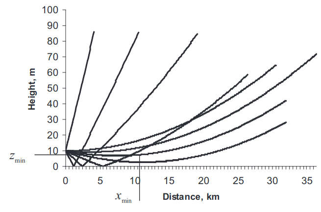
As observed from Eq. (49) the values of E satisfying the inequality E ≤ μ³ z₀ determine the real hit-angles ϑ, those, in turn, represent uniform plane waves with angle ϑ/m between the normal to their wavefront and tangential to the radius r = α+z₀ at the point of source location. Trajectory (48) has a minimum in:

$x_{min}=\frac{2k}{{\mu }^3}\sqrt{{\mu }^3{z}_0–E} \mathrm{and} z_{min}\left(x_{min}\right)=\frac{E}{{\mu }^3}.$

From that it follows that the values E < 0 determine the waves reflected from the earth’s surface. The sector

$–\alpha \tan \left(\sqrt{k{z}_0/m^3}\right)<\vartheta <a \tan \left(\sqrt{k{z}_0/m^3}\right)$

determines the “space” rays (direct wave) related to a stationary value of E from the interval:

$0<E<{\mu }^3{z}_0.$

The ray trajectories described by Eqs. (47) and (48) are shown in Figure.

Therefore, in the line-of-sight region, i. e.

$x<\sqrt{2\alpha }\left(\sqrt{z}+\sqrt{z_0}\right)$

we can select two areas of integration in Eq. (2.43):

$I_1={\int }_{–\infty }^{0}dE{\Psi }_E\left(z\right){\Psi }_E^{*}\left(z_0\right)e^{j\frac{E}{2k}x}, Eq. 50$

$I_2={\int }_0^{\infty }dE{\Psi }_E\left(z\right){\Psi }_E^{*}\left(z_0\right)e^{j\frac{E}{2k}x}, Eq. 51$

Let us substitute Eqs. (45)–(47) into Eq. (51) and assume z > z₀ and:

$k{z}_0/m\gg 1. Eq. 52$

The integration in Eq. (51) can be performed using the method of stationary phase. The result is given by:

$I_1=\theta \left(\sqrt{2\alpha }\left(\sqrt{z}–\sqrt{z_0}\right)–x\right)I_{11}+I_{12}, Eq. 53$

$I_{11}=2\mu A^2\sqrt{\frac{2k\mathrm{\pi }}{x}}exp\left\{–j\frac{\mathrm{\pi }}{4}+j\frac{k}{2x}{\left(z–z_0\right)}^2+j\frac{kx}{2\alpha }\left(z+z_0\right)–j\frac{1}{12}{\left(\frac{mx}{\alpha }\right)}^3\right\},$

$I_{12}=\sqrt{\frac{k}{\alpha }}\frac{\sqrt{–\xi }}{4\sqrt{\mathrm{\pi }}}\frac{1}{\sqrt[4]{z{z}_0}}·exp\left\{j{\left(\frac{k}{m}\right)}^{3/2}\left(z^{3/2}+z_0^{3/2}\right)+j\frac{kx}{2\alpha }\left(z+z_0\right)–j\frac{1}{12}{\left(\frac{m\xi }{\alpha }\right)}^3\right\} Eq. 54$

where

$\xi =x–\sqrt{2\alpha }\left(\sqrt{z}+\sqrt{z_0}\right).$

Consider integral (52) and make use of the asymptotic expression for Airy functions w_1,2 (E/μ²) for large positive arguments:

$w_1\left(\frac{E}{{\mu }^2}\right)\approx w_2\left(\frac{E}{{\mu }^2}\right)\approx {\left(\frac{E}{{\mu }^2}\right)}^{1/2}exp\left(\frac{2}{3{\mu }^3}{E}^{3/2}\right). Eq. 55$

Substituting Eq. (55) into Eq. (45) we obtain S(E) = 1. Let us introduce the Airy function v(t) by the relationship:

$2j\nu \left(t\right)=w_1\left(t\right)–w_2\left(t\right) Eq. 56$

and the variable τ = E/μ²-μz₀. The integral (52) can then be transformed into:

$I_2\approx \frac{1}{4\mathrm{\pi }}{e}^{j\frac{x}{2k}{\mu }^3{z}_0}{\int }_{–\mu z_0}^{\infty }{e}^{j\frac{x\tau }{2k}{\mu }^2}\nu \left(\tau \right)\nu \left(\tau –\mu \left(z–z_0\right)\right)d\tau . Eq. 57$

Without significant error the low limit in the integral (58) can be extended to -∞. Substituting into Eq. (58) the integral representation for ν(t):

$\nu \left(t\right)=\frac{1}{2\sqrt{\mathrm{\pi }}}{\int }_{–\infty }^{\infty }exp\left(j\frac{{\xi }^3}{3}+j\xi t\right)d\xi Eq. 58$

and performing the integration, we obtain:

$I_2\approx \sqrt{\frac{k}{2\mathrm{\pi }x}}exp\left\{–j\frac{\mathrm{\pi }}{4}+j\frac{k}{2x}{\left(z–z_0\right)}^2–j\frac{kx}{2\alpha }\left(z+z_0\right)–j{\left(\frac{mx}{\alpha }\right)}^3\right\}. Eq. 59$

Equation (60) describes the direct wave in the range of distances:

$\sqrt{2\alpha }\left(\sqrt{z}–\sqrt{z_0}\right)<x<\sqrt{2\alpha }\left(\sqrt{z}+\sqrt{z_0}\right)$

and transforms into Eq. (53) with

$x=\sqrt{2\alpha }\left(\sqrt{z}–\sqrt{z_0}\right)$

. Therefore in a whole line-of-sight region the Green function (41) can be represented by superposition of the direct wave and the wave reflected from the earth’s surface.

Let us consider the Green function’s representation (41) in a shadow region, i. e.

$x>\sqrt{2\alpha }\left(\sqrt{z}+\sqrt{z_0}\right).$

In this case the contour of integration over dE can be closed in the upper half-plane and the integral is represented by a residue sum over the poles of S(E). In the particular case of normal refraction and ideal boundary conditions, the poles are given by:

$w_1\left(\frac{E}{{\mu }^2}\right)=0 \mathrm{and} E_n=\frac{k^2}{m^2}{\tau }_n{e}^{j\mathrm{\pi }/3}, {\tau }_1=2,338, {\tau }_2=4,02, ... Eq. 60$

As a result, we obtain the Green function representation in terms of the normal wave series:

$G\left(\overrightarrow{r}, {\overrightarrow{r}}^{\prime }\right)=\sqrt{\frac{2\mathrm{\pi }}{k\left(x–x^{\prime }\right)}}exp\left\{j\frac{\mathrm{\pi }}{4}+j\frac{k}{2}\frac{{\left(\gamma –{\gamma }^{\prime }\right)}^2}{x–x^{\prime }}\right\}·\sum _{n=1}^{\infty }exp\left(j\frac{E_n}{2k}\left(x–x^{\prime }\right)\right)\frac{w_1\left({\displaystyle \frac{E}{{\mu }^2}}–\mu z\right)}{w_1^{\prime }\left({\displaystyle \frac{E}{{\mu }^2}}\right)}\frac{w_1\left({\displaystyle \frac{E}{{\mu }^2}}–\mu z^{\prime }\right)}{w_1^{\prime }\left({\displaystyle \frac{E}{{\mu }^2}}\right)}. Eq. 61$

In conclusion, the Green function has been built as an expansion over the set of complete and orthogonal eigenfunctions of the continuous spectrum. In the case of normal refraction, such a representation produces final formulas for the field of the point source that are similar to those introduced by Fock on the basis of the classical approach of the contour integral.

It is worthwhile to emphasise the purpose of the above presentation for a Green function. In a problem of multiple scattering the whole path is involved in the scattering process and one needs to have a representation for the field (or Green function) which is equally applicable in the line-of-sight and shadow regions. Also, in the process of obtaining the closed set of equations for statistical moments of the field, the Green function has to possess some properties of orthogonality and completeness which can be achieved by using the above expansion over the set of eigenfunctions of the continuous spectrum.

Author

Olga Nesvetailova

Freelancer

Literature

1. Fock, V.A. Electromagnetic Diffraction and Propagation Problems, Pergamon Press, Oxford, 1965.
2. Fock, V.A. Distribution of currents excited by a plane wave on the surface of conductor, J. Exp. Theor. Phys., (Nauka), 1945, 15 (12), 693–702.
3. Leontovitch, M.A. Method of solution to the problems of em wave propagation over the boundary surface, Izv. Acad. Nauk, Ser. Fiz., 1944, 8 (1), 16–22.
4. Leontovitch, M.A., Fock, V.A. Solution to a problem of em wave propagation over the Earth’s surface using the method of parabolic equation, J. Exp.Theor. Phys., (Nauka), 1946, 16 (7), 557–573.
5. Fock, V.A. Theory of wave propagation in a non-uniform atmosphere for elevated source, Izv. Acad. Nauk, Ser. Fiz., 1960, 14 (1), 70–94.
6. Krasnushkin, A.E. The expansion over normal waves in a spherically-stratified medium, Dokl. Acad. Nauk SSSR, 1969, 185 (6), 1262–1265.
7. Kravtsov, Yu.A., Orlov, Yu.I., Geometric Optics of Non-uniform Media, Nauka, Moscow, 1980, 340 pp.
8. Rotheram, S. Radiowave propagation in the evaporation duct, The Marconi Rev., 1974, 67 (12), 18–40.
9. Booker, H.G., Walkinshaw W. The mode theory of tropospheric refraction and its relation to waveguides and diffraction, in Meteorological Factors in Radiowave Propagation, The Royal Society, London, 1946, pp. 80–127.
10. Andrianov, V.A. Diffraction of UHF in a bilinear model of the troposphere over the Earth’s surface, Radiophys. Quantum Electron., 1977, 22 (2), 212–222.