Delve into Loran-C Millington’s Method and its application in calculating propagation delays using conductivity data.
This article covers the importance of conductivity as a key parameter, detailed calculations, and the computer implementation of Millington’s Method.
Introduction
Calculation of the propagation behavior of radio waves over mixed paths (includingvarious types of terrain and seawater) to estimate ASFs is both theoretically complex and numerically tedious. This appendix presents a simplified description of one commonly used empirical approach for ASF calculation known as Millington’s Method.
The Loran-C System: A More Detailed ViewThis article discussed the overall approach for calculating the time required for a loran groundwave signal to propagate from a transmitter to the vessel or aircraft over a distance, d. To a first approximation, the time to propagate this distance is simply the distance divided by the speed of light through the atmosphere (Primary PhaseFactor). Although this simple calculation is nearly correct, it is not sufficiently accurate to satisfy the absolute accuracy requirements of the Loran-C system. Two additional corrections are usually applied to this simple formula for calculation of TDs.
The first, termed secondary phase factor (SF), corrects for signal propagation delays over seawater compared to propagation through the atmosphere. The second, termed additional secondary factor (ASF), corrects for the additional signal propagation delay over a mixed land seawater path compared to an all-seawater path. Traditionally, these corrections are calculated as increments to be added algebraically (i. e., with regard to sign) to the time computed from the “simple” model (PF). That is, the propagation time required to traverse a distance, d, is first calculated based upon propagation through the atmosphere. Next, increments to this time (SF) and (ASF) are calculated and added to the propagation time.
Conductivity -A Key Parameter
The conductivity, denoted by the symbol σ, is a key determinant of the magnitude of the SF and ASF corrections. Conductivity is measured in units of mhos/meter or in millimhos/meter (1 000 millimhos is equal to 1 mho). The unit “mho,” is ohm spelt backwards and captures the reciprocal relationship between resistivity and conductivity.
Table F-1 provides a sample of conductivity values for seawater and various types of terrain.
| Table 1. Conductivity values | |
|---|---|
| Terrain Description | Conductivity in Millimhos/meter σ |
| Seawater | 5 000 |
| Rich agricultural land | 10-30 |
| Forested land | 8 |
| Fresh water | 8 |
| Pastoral land, medium hills and forestation | 4-5 |
| Rocky land, dry sandy coastal land | 2 |
| Mountainous land, cities | 1 |
| Snow-covered mountains | 0,5 |
Calculation of Propagation Delays From Conductivity Data
The incremental propagation time (compared to the travel time through the atmosphere) for homogeneous paths is a function of distance and can be determined using generalized curves found in National Bureau of Standards (NBS) Circular 573. An extract from these curves is reproduced in Figure 1 This set of curves has been simplified for reproduction purposes. Only three types of propagation surface are included. The actual NBS diagram has data for numerous conductivity values included.x.
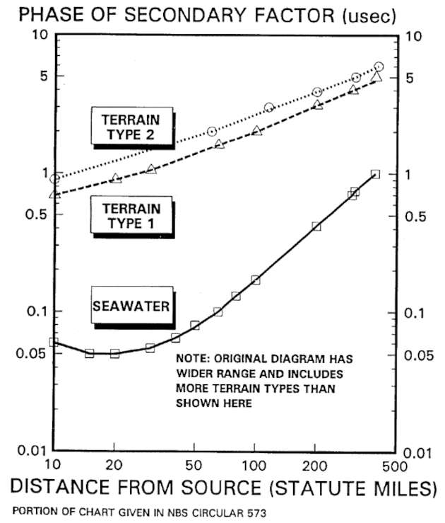
This figure shows the additional propagation time (phase of the secondary factor) in usec as a function of the distance of the receiver from the transmitter. This illustration includes estimates for an all-seawater path, and also homogeneous paths across two different types of terrain with lower conductivity.
To illustrate, the incremental propagation time (over that calculated employing the velocity of light through the atmosphere) for a signal to propagate a distance of 390 statute miles (SM) over an all-seawater path would be approximately 1 usec, referring to the “seawater” path curve in Figure 1 The SFs for the seawater path can also be calculated from equations (11-6) and (11-7) given in the main text.x.
Conductivity Data
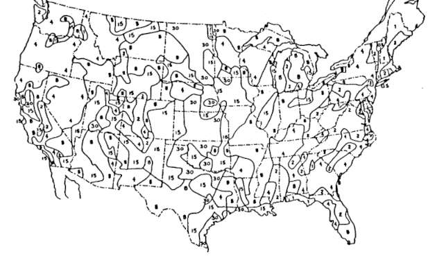
Calculation of these time increments requires a data base of conductivity estimates across all possible land and seawater paths. Figure 2 shows these estimates (in millimhos/meter) for the continental United States.
Use of Conductivity Data in Millington’s Method
Figure 3 shows the computational steps in the use of Millington’s Method. This procedure will be illustrated with a numerical example.
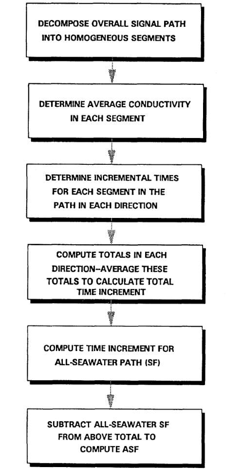
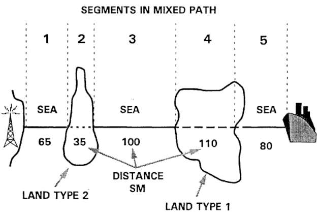
The first step is to decompose the overall path from transmitter to receiver into a series of homogeneous segments – each with the same conductivity value. Figure 4 shows an illustrative path from a loran transmitter over seawater and two islands, each with a different terrain type. In this case there are a total of five segments in the path, three over seawater, and two over islands of different terrain type.
The second step shown in Figure 3 is to determine the average conductivity in each segment. The average conductivity for the seawater segments is 5 000 millimhos/meter. Average conductivities for the various terrain types can be found in tables similar to Table 1 or generalized diagrams similar to Figure 2.
The third step shown in Figure 3 is to compute the propagation time increments for each segment of the path in each direction. Consider first the direction from the transmitter to the vessel in Figure 4. Table 2 shows the equations necessary for computation of these time increments in both directions for a five-segment path.
| Table 2. Notation for composite baseline analysis |
|---|
 |
- The first segment is over seawater, a distance of 65 statute miles (SM). Reference to Figure 1 (or exact computations using the seawater equations in The Loran-C System: A More Detailed Viewthis article) indicates that the time increment for this segment is approximately 0,1 usec.
- The second segment is over land of terrain type 2 from 65 miles (at the left endpoint) to 100 miles (at the right endpoint). To calculate the time increment, read from Figure 2 (Type 2 terrain) the time increments associated with the left endpoint (1,6 usec) and the right endpoint (2 usec). The time increment, 0,4 usec in this example, is the difference between these two values.
- The third segment in Figure 4 is an all-seawater path 100 statute miles in extent, with a left endpoint of 100 miles and a right endpoint of 200 miles. The propagation time increments (Figure 1) are 0,18 usec and 0,41 usec, respectively, an increment for this segment of 0,23 usec.
- The fourth segment is over terrain Type 1, with a left endpoint of 200 miles and aright endpoint of 310 miles. The corresponding time increments are approximately 3,2 usec and 4,3 usec, a difference of 1,1 usec.
- The final segment is over seawater, from 310 to 390 statute miles. The time increment for this seawater segment is approximately 1,01 usec (at 390 statute miles) less 0,74 usec (at 310 statute miles), a difference of 0,27 usec.
The fourth step in Figure 3 is to compute the total time increments in each direction. The total time increment from left to right is 0,1+0,4+0,23+1,1+0,27 = 2,1 usec. If the direction of calculation were reversed, an identical series of computations would lead to a total time increment of approximately 2,3 usec. The computational procedure is to average these calculations to estimate the time increment.
The need to consider propagation along both directions of the pathway relates to the principle of reciprocity. This principle states that in a linear uniform propagation medium, the response of the medium to a source is unchanged when the source and the receiver are interchanged. The direction of a path from a source across a medium does not affect the response of the medium. As shown above, Millington’s method predicts a phase delay by computing a correction from source to transmitter and a reciprocal correction. The values of these corrections are averaged. Except in the unlikely case where the path and its reciprocal are identical, the two time increments calculated in each direction are not identical, because the conductivity segments are biased, depending upon their proximity to the source.
This average, 2,2 usec in this example, is the total increment to propagation time compared to an atmospheric signal path. Recall that the additional secondary factor is defined as the incremental time over and above an all-seawater path.
The fifth step in Figure 3 is to compute the SF for the entire path. Using either Figure 1 or the equations given in The Loran-C System: A More Detailed Viewthis article, the SF for the signal to propagate 390 statute miles over seawater would be 1,01 usec.
Read also: Loran-C Position Determination and Accuracy
The final step shown in Figure 3 is to subtract the time increment for an all-seawater path from the average total increment to calculate an ASF. The ASF in this case would be 2,20-1,01 = 1,19 usec.
The ASF calculated above applies to the propagation path from one transmitter to one location in the coverage area. The ASF appropriate to a loran TD LOP involves two propagation paths, one from the master to the user’s location, the other from a secondary to the user’s location. Therefore, to calculate the ASF corresponding to a particular master station pair, it is necessary to make the above calculations for both paths, and subtract the individual ASFs to calculate an ASF for a TD at that point in the coverage area.
Careful examination of Figure 1 (or the original curve from which this extract was taken) indicates that the curves of propagation delays for various types of terrain are generally above that for seawater – that is, land slows loran waves even more than water. The ASF calculated for a single path will generally be either zero (if the path is an all seawater path) or positive (if the path involves segments over both water and land). However, the ASF for a master-secondary pair could be either positive or negative, depending upon the propagation characteristics for the paths from the user’s location to the master and secondary. This is why the ASF correction tables contain both positive and negative quantities – to a first approximation entries will either be positive or negative depending upon the relative portion of the paths from secondary or master that are over land versus seawater.
Reference to Figure 4 shows why ASFs sometimes appear to change in a discontinuous manner. Imagine, for example, that the path between the transmitter and the user were swung through an arc. As soon as the path were clear of the islands, the ASFs would go abruptly to zero. Lack of smoothness of the ASF curves (and the reason why these curves are not easily interpolated) relates (among other things) to lack of smoothness of terrain features.
In practice, these predictions would be validated with survey data, and ASF tables and loran overprinted charts adjusted based upon survey data.
Computer Implementation
In order to produce ASF tables, it is necessary to replicate the computational procedure used here many times over a latitude-longitude grid. As these computations are numerically tedious, computers are used to produce the tables of ASF values. Readers interested in details of these computer programs can refer to Speight (1982).

- Abramowitz, M., et al. “Approximate Method for RapidLoran Computation,” Navigation; Journal of the Institute of Navigation, Vol. 4, No. 1, March 1954, pp. 24-27.
- Alexander, G. “The Premier Racing Tool,” Ocean Navigator, Issue No. 20, Jul/Aug 1988, pp. 37, er seq.
- Anonymous. “Loran: Installation Pitfalls, and How Friendly Should Your Loran Be?” Practical Sailor, Vol. 11, No. 24, December 15, 1985, pp. 1, et seq.
- Anonymous. Manual on Radio Aids to Navigation, International Associationof Lighthouse Authorities, Nouvelle Adresse, 13 Rue Yvon-Villarceau 75 116, Paris, 1979.
- Appleyard, S. F. Marine Electronic Navigation. Routledge and Kegan Paul Ltd., Boston, MA, 02108, 1980.
- Ashwell, G. E., B. G. Pressey, and C. S. Fowler. The Measurement of the Phase Velocity of Ground Wave Propagation at low Frequencies Over a Land Path. Proceedings of the Institute of Electrical Engineering (London) 100 Part III, 1953.
- Bedford Institute of Oceanography. Loran-C Receiver Performance Tests, Bedford Institute of Oceanography, P. O. Box 1006, Dartmouth, NovaScotia, Canada, B2Y 4A2.
- Blizard, M. M. et al. Harbor Monitor System Final Report, CG-D-17-87, ADA 183 477, Dec. 1986, Available through the National Technical Information Service, Springfield, VA, 22161.
- Blizard, M. M., Lt. and CWO 3 D. C. Slagle. Differential Loran-C System Final litter, Draft, United States Coast Guard, January 1987.
- Blizard, M. M. and D. C. Slagle, “Loran-C West Coast Stability Study,” Proceedings of the Fourteenth Wild Goose Technical Symposium, Wild Goose Association, Bedford, MA, 1985.
- Brogdon, B., “Loran Expansion,” Ocean Navigator, Issue No. 42, SeptfOct 1991, pp. 87, et seq.
- Brogdon, W. “Loran Hook, a Little Known, Foible Explained,” Boating, August 1991, p.42.
- Brogdon, W. “Electronic Errors,” Ocean Navigator, Issue No. 40, June 1991,pp. 70, etseq.
- Brogdon, W. “Pathfinders,” American Hunter, Vol. 19, No. 7, July 1991.
- Burt, W. A., et al. Mathematical Considerations Pertaining to the Accuracy of Position, Location, and Navigation Systems, Part I, Stanford Research Institute, 1966. Available from National Technical Information Service, AD-629609, US Department of Commerce, 5825 Port Royal Road, Springfield, VA 2215 1.
- Canadian Coast Guard, Aids and Waterways Branch. A Primer on Loran-C, Ottowa, Ontario, Canada, 1981.
- Connes, K. The Loran, GPS & NAVICOMM Guide, Butterfield Press, 1990.
- Culver, C. “A New High Performance Loran Receiver,” Proceedings of the Sixteenth Annual Technical Symposium, The Wild Goose Association, 20-27 October 1987, pp. 282, et seq.
- Dahl, B. “Adopting Loran-C to Everyday Navigation,” Cruising World,May 1983,pp. 40-45.