Delve into the world of LORAN-C in this detailed article, covering essential aspects such as position determination, accuracy factors, and the impact of atmospheric and man-made influences.
- Introduction
- Position Determination Using TDs
- Loran Accuracy
- Determinants of Loran-C Accuracy
- Stability of the Transmitted Signal
- Atmospheric and Man-Made Effects on Propagation
- Factors Causing Temporal Variability
- Factors Associated With Spatial Variability
- Other Factors
- System Geometry
- Crossing Angles
- Gradient
- Brief Remarks on Station Placement
- Putting it Together: drms
- Accuracy vs. Location in the Coverage Area
- Coverage Diagrams
- Chain Selection
- Practical Pointers
Explore system geometry, coverage diagrams, and practical tips for optimizing LORAN-C performance in various applications.
Introduction
This article shows how positions are identified using Loran-C, examines the important topic of Loran-C accuracy and its determinants, and briefly notes how range limits and coverage diagrams are developed for this system. Actual plotting of positions, including the use of loran linear interpolators, is addressed more fully in Loran-C Charts and Related Information“Loran-C Charts Key Components and Navigation Techniques”. Although some of the material in this chapter is unavoidably technical, the information presented here is very important to mariners and other users who need to know the capabilities of the loran system, and how to exploit these capabilities in full measure. Coast Guard and Coast Guard Auxiliary experience in dealing with thousands of search and rescue cases annually indicate that many mariners use loran without full knowledge of its capabilities or limitations. Some mariners have excessively optimistic expectations for the accuracy of the system and little knowledge of how accuracy varies throughout the coverage area – thereby facing increased risk of grounding or other navigational mishaps (see Humber, 1991 for an illustrative sea story). Yet others realize some of these limitations, but are unaware of techniques to take full advantage of the system – thereby sacrificing efficiency and utility.
The principal reason for including the material in this chapter is that this information is important. A subsidiaryreason is that the subject of accuracy and its determinants is generally eitheromittedentirely or treatedin only a sketchy manner in many texts and/or the owners manuals that accompany loran receivers – including those manufactured by some of the leading companies. It can be arguedrightly that the loran user need not be a scientist or engineer in order to operate a loran set, but it is equally true that a knowledge of the basic technical principles of this system is essential to safe and efficient navigation.
Position Determination Using TDs
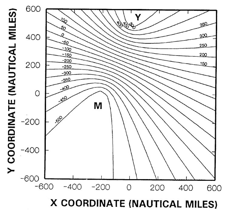
As noted in The Loran-C System: A More Detailed View“Understanding Loran Transmitters and Hyperbolic Systems”, differential distances or TDs from a station pair determine a “family” or set of hyperbolic LOPS (see, for example, Figure The Loran-C System: A More Detailed View“A more conventional depiction of Loran LOPS”). Knowledge of even one loran TD can be useful (e. g., by crossing it with a visual or radar bearing or range to determine a fix) but, more typically, TDs from two station pairs are used for fixing a user’s position. Figure 1, for example, shows the same geographic plane and master station used for illustration in Figure The Loran-C System: A More Detailed View“A more conventional depiction of Loran LOPS”. This figure shows the differential distances from the master station, assumed to be located at the point (-200, 0), arid the Yankee secondary, assumed to be located at the point (0, 500) in the rectangular grid. Again the familiar pattern of hyperbolic LOPS is shown in Figure 1, except that this figure presents the difference in distance of the LOPS for the master-Yankee station pair rather than the master-Xray pair.
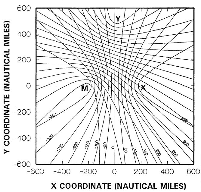
If both the master-Xray and master-Yankee station pair time differences are considered, the individual sets of loran LOPS (shown in Figure The Loran-C System: A More Detailed View“A more conventional depiction of Loran LOPS” and Figure 1) can be superimposed to determine the hyperbolic lattice illustrated in Figure 2. (The term hyperbolic grid is also commonly used, but because the axes of a grid are typically at right angles, the word “lattice” is preferable.) As can be seen clearly in Figure 2, the LOPs from the two station pairs do not always cross at right angles.
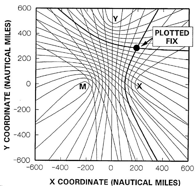
As shown below, the crossing angle of the LOPs is an important determinant of fix accuracy.) Position determination is simply a matter of locating the LOPs represented by each measured time difference (i. e., those from each of two master-secondary pairs) and fixing the users position at the intersection of these two LOPs on the hyperbolic lattice, as illustrated in Figure 3.
Loran-C TDs for various chains are displayed on special charts, termed loran overprinted charts. Loran fixes can be converted from TD units to latitude and lon gitude using these charts, or plotted directly.
Were the LOPs straightlines (on the plane), two LOPs (not parallel) would intersect at only one point. However, two hyperbolic LOPs can, in certain circumstances, intersect at two points in the coverage area of the chain. This phenomenon is illustrated in Figure 2. Look carefully at where the “350” Xray LOP crosses the Yankee LOP near the Xray secondary in Figure 2. One crossing is evident just northwest of the Xray secondary, and another is shown some distance southeast of this secondary at the edge of the diagram-so there are two possible positions on this chart with exactly these same TDs. Absent other information, a mariner would not know which of these positions is correct. This problem, termed fix ambiguity, occurs only in the vicinity of the baseline extensionof any master-secondary pair.
Although some Loran-C receivers can warn the user of this problem with an ambiguity alarm (and yet other, more sophisticatedreceivers, are programmed to track three secondaries and automatically resolve this ambiguity), the safest course of action is to avoid use of any secondary station in the vicinity of its baseline extension. In practice, the navigator would switch to another secondary in lieu of Xray in this illustration, and the ambiguity would be resolved.
Referring to Figure 2, note also that the crossing angle of the two sets of TDs is very small in the area south of the Xray secondary. In fact, the two setsof LOPS are very nearly parallel in this area. Such small crossing angles are incompatible with accurate fixes. This important characteristic of LOPS is discussed at some length below. For the present, however, suffice it to say that the accuracy of a loran fix depends (among other things) upon the user’s position with respect to the transmitters.
Avoid use of loran stations in the vicinity of their baseline extensions. Fix accuracies are substantially degraded, and ambiguous positions may result.
Loran-C TD LOPS for various chains and secondaries are printed on special nautical charts, termed loran overprinted charts, as discussed in Loran-C Charts and Related Information“Loran-C Charts Key Components and Navigation Techniques”. Each of the sets of LOPs (often termed rates, although technically a rate refers to both the GRI and the secondary) is given a distinct color (e. g., on US nautical charts, the color blue is used to print TDs for the Whiskey secondary, magenta for the Xray, black for the Yankee, and green for the Zulu) and denoted by a characteristic set of symbols or label to depict the LOP Usersshould be careful to note the GRI designator as well as the color of the overprinted LOP. This is because some charts (in areas of overlappingchain coverage)may have more than one family of LOPs printed in the same color if the same secondary (e. g., the Zulu secondary) from more than one chain can be received.x. For example, a magenta Loran-C overprinted LOP might be labeled 9960-X-25750 on the nautical chart. Decoded, this particular label means that the chain GRI designator is 9960, the TD for the master-Xray station pair is being plotted, and the estimated time difference along this LOP is 25,750 microseconds.
If each and every LOP from this station pair were shown on the chart, a very cluttered (indeed, virtually unusable) chart would result. For this reason, only selected LOPS are printed, e.g. 25750, 25760, 25770 microseconds, etc. (the interval varies with the station pair and the scale of the chart), and the GRI designator and station pair are shown only on selected (e. g., every fifth) LOPs. In the typical case where the measured TD is not shown exactly on the chart – for example, if the TD displayed on the loran receiver were 25 755,5 – it would be necessary to interpolate between the charted LOPs. This interpolation process is explained and illustrated in Loran-C Charts and Related Information“Loran-C Charts Key Components and Navigation Techniques” and is quite simple in practice, using the “Mark I human eyeball” or, for greater accuracy, the loran interpolator printed on the chart, or a special purpose interpolator (made of plastic or cardboard) available from commercial sources or the Coast Guard.
A given loran overprinted chart may have three or more secondaries (from one or more chains) displayed if usable signals can be received from several station pairs in the area covered by the chart. The user has the option of selecting from among several TDs (stationpairs) for position determination. In this situation, chains and master-secondary pairs should be selected to provide reliable signal reception and to maximize the accuracy of the resulting fix. Criteria for selection of chains and station pairs are presented in this chapter, following the discussion of loran accuracy.
Because of overlapping coverage of Loran-C chains and/or secondaries within a chain, the user often has a choice among rates (TDs). Criteria for selection of the “best” secondaries are presented later in this article.
Incidentally, the displays of most loran receivers do not use letter designators to identify the TDs for each station pair. Rather these receivers use numerals to display the particular TDs, e. g., “TD1,” “TD2,” etc. Because of the manner in which CDs are selected, the identification of the specific station pairs is generally obvious from the magnitude of the TDs. However, the owners manuals accompanying the receiver typically provide a code to indicate the correspondence between the TD’s displayed and the letter designation for the secondaries. For example, Raytheon’s RAYNAV 570 receiver uses the code “1 = Whiskey,” “2 = Xray,” etc. to denote the secondaries of the 9960 chain. Be careful to consult the correct entry in the correspondence table, as different codes may be appropriate for each chain.
Loran Accuracy
Accuracy is one of the least understood attributes of the Loran-C system. To begin, there are three major types of accuracy relevant to a navigation system:
- predictable accuracy,
- repeatable accuracy,
- relative accuracy.
There are three types of accuracy relevant to the Loran-C system; absolute accuracy, repeatable accuracy, and relative accuracy. Absolute and repeatable accuracy are most relevant to the majority of users.
Predictable (also called absolute or geodetic) accuracy is the accuracy of a position with respect to the geographic or geodetic coordinates of the earth. For example, if a mariner were to note the TDs corresponding to a charted object (e. g., a light house on a “Texas tower“) and travel to the point indicated by these time references only, the difference between the vessel’s loran-determined position and the actual location of the lighthouse would be a measure of the absolute accuracy of the system.
Repeatable accuracy is the accuracy with which a user can return to a position whose coordinates have been measured at a previous time with the same navigational system. Continuing the above example, if the mariner were to travel to the light tower referenced above, note the Loran-C TDs corresponding to the actual position of the structure, and later return to these same TDs (rather than the TDs corresponding to the coordinates shown on the loran overprinted chart), the resulting position difference would be a measure of repeatable accuracy. Note that TDs for many locations of interest to the mariner (e. g., light structures, day markers, channel turnpoints or centerlines, wrecks, etc.) are sometimes published by the Coast Guard and/or commercial sources. If these TDs are developed from actual survey data (as in the case for those published by the Coast Guard) rather than simply read from a chart, the accuracy of these coordinates approaches the repeatable accuracy, rather than the absolute accuracy, of the system (see below). To many users, repeatable accuracy is more important than absolute accuracy – exploitation of the great repeatable accuracy of Loran-C enables the user to take full advantage of the capabilities of this navigation system.
Finally, relative accuracy is the accuracy with which a user can measure position relative to that of another user of the same navigation system at the same time. Applications where relative accuracy is important (e. g., search and rescue) are more specialized and not addressed here.
Types of Loran-C accuracy:
- absolute,
- repeatable,
- relative.
Of these three types of accuracy, most users are concerned with either absolute or repeatable accuracy. Loosely stated, the absolute accuracy of the system includes both the precision (random errors) and the bias (systematic errors) of the system, whereas the repeatable accuracy of the system includes only the random errors of the system. Both types of accuracy (i. e., absolute and repeatable) are important to loran users, but for different purposes. For example, a mariner entering an unfamiliar harbor and trying to locate the sea buoy marking this initial approach fix to this harbor would be concerned with the absolute accuracy of the Loran-C system. However, if the mariner had visited the harbor (on previous occasions) and recorded the actual TDs corresponding to the sea buoy, repeatable accuracy would be at issue. Likewise, repeatable accuracy is relevant to a fisherman returning to a previously visited area and seeking to locate a productive wreck, to avoid “hangs” or other bottom obstructions that could foul nets, or to find lobster pots in poor visibility.
This distinction between absolute and repeatable accuracies is quite important, because the system accuracy differs depending upon how accuracy is defined. The absolute accuracy of the Loran-C system varies from approximately 0,1 to 0,25 nautical miles, depending upon the mariner’s location in thecoverage area. This assumes that overland propagation delays, ASFs, are employed for correcting observed TDs. The official specification of the Loran-C system is that absolute accuracy should be no less than 0,25 nautical mile within the defined coverage area of the chain. There is no explicit specification for the repeatable accuracy of Loran-C, although a range of from 60 ft to 300 ft is noted in the Federal Radionavigation Plan. Repeatable accuracy also depends upon the mariner’s location in the coverage area.
The absolute accuracy of Loran-C varies from 0,1 NM to 0,25 NM. Repeatable accuracy is much greater, typically from 60 ft to 300 ft.
The high repeatable accuracy of Loran-C enables advantageous use of this system for selected harbors and harbor approaches (HHA) (also termed harbors and harbor entrances, HHE) where TD data have previously been collected and recorded. When the repeatable capabilities of Loran-C are exploited, this system can be employed as a secondary system in HHA navigation. Mariners are cautioned, however, never to rely solely on any one navigation system – particularly in areas where precision navigation is important.
The repeatable accuracy of Loran-C can be used to advantage in HHA navigation to supplement other systems for fixing a vessel’s position. Mariners are cautioned never to rely solely on one system.
Determinants of Loran-C Accuracy
Several factors collectively determine the overall accuracy (repeatable or absolute) of the Loran-C system. For example, transmitters, transmitter controls, the medium through and over which the signals travel, receivers, charts, and the user determine the overall accuracy of the system. Each component contributes to the system error – these sum statistically to yield the overall system error.
Table 1 identifies the most important sources of error (absolute or repeatable) in the operation and use of the Loran-C system. Some factors affect both absolute and repeatable accuracy, while others affect only absolute accuracy. All of these factors, save operator error, are included in the accuracy specifications noted above. Human error includes a myriad of errors and blunders, such as misreading charts, receiver displays, transposing digits in copying positions, applying ASF corrections with the wrong sign, misreading tables, etc. Because of the diversity of these errors and their inherent unpredictability, human errors are typically not quantifiedin the system accuracy specifications. This does not mean that these errors are unimportant or that the user should not take pains to minimize these errors.
| Table 1. Selected factors limiting the accuracy of Loran-C position determination | ||
|---|---|---|
| Factor | Effect On | |
| Geodetic Accuracy | Repeatable Accuracy | |
| Crossing Angles and gradients of the Loran-C LOPs | Yes | Yes |
| Stability of the transmitted signal (e. g., transmitter effect) | Yes | Yes |
| Loran-C chain control parameters | Yes | Yes |
| Atmospheric and man-made noise | Yes | Yes |
| Factors with temporal variations in signal propagation spread (e. g., weather, seasonal effects, diurnal variation, etc.) | Yes | Yes |
| Accuracy with which LOPs are printed on nautical charts | Yes | No |
| Sudden Ionic Disturbances | Yes | Yes |
| Accuracy of computer algorithms for coordinate conversation | Yes | No |
| Shipboard noise | Yes | Yes |
| Receiver quality and sensitivity | Yes | Yes |
| Operator error | Yes | Yes |
The first entry in Table 1 (crossing angles and gradients of the Loran-C LOPS) includes a variety of terms usually grouped under the rubric of “Geometric Factors.” These important determinants of accuracy are discussed in some detail later in this chapter. The balance of the error sources shown in this table are summarized briefly below.
Stability of the Transmitted Signal
This term refers to the errors of the system associated with loran transmissions. Although the loran transmitters produce highly accurate pulsed signals, there is a small variability from this source, termed transmitter effects. At some LORSTAs equipped with tube-type transmitters, redundant transmitters are switched in and out as part of routine maintenance activities, resulting in small signal perturbations. This error will decline in importance as solid-state transmittersare employed throughout the chains. As of this writing, only the West Coast Chains, LORSTAs Dana, IN, and Cape Race, NFLD employ tube-type transmitters. Additionally, LORSTA operators make routine manual phase adjustments (MPAs) to the signal in order to maintain the signal within preestablished tolerances. Additionally, Local Phase Adjustments (LPAs) are made to compensate for differences in cesium oscillator drift.
Another signal perturbation (termed chain control effect) results when a control monitor station becomes inoperative, and alternative control schemes are used (e. g., a switch fromone monitor location to another). This shift “warps” the loran lattice slightly, and contributes to variability of the loran signal.
Atmospheric and Man-Made Effects on Propagation
Atmospheric conditions can significantly affect the propagation of the Loran-C signal, and derivatively of the accuracy of the fix. (Noise also affects the signal-to-noise ratio (SNR) and the maximum distance at which a usable signal can be received, as discussed below.) Atmospheric noise is the dominant form of noise in the loran band. It is produced by lightning all over the earth. Atmospheric noise is always present, because thunderstorms are always present. Each lightning strike produces a point noise source – the effects of this noise depend upon the distance from the storm to the receiver. Atmospheric noise is generally greater in the summer than the winter, and in the tropics compared to the higher latitudes.
Factors Causing Temporal Variability
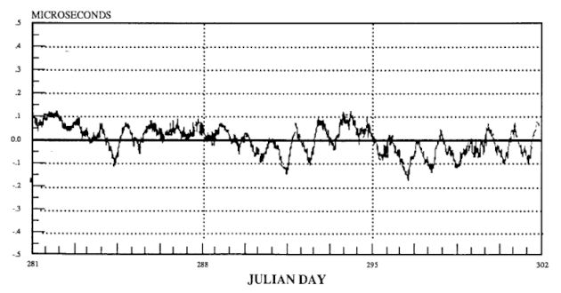
There are several factors that can cause temporal variation in signalpropagation throughout the system coverage area. Recall (from The Loran-C System: A More Detailed View“Understanding Loran Transmitters and Hyperbolic Systems”) that ASFs vary with the characteristics of the mixed land-sea path that loran signals travel to the observer. Terrain moisture and temperature, for example, exhibit seasonal variability which, in turn, affects signal propagation (seasonal effect). Figure 4, for example, shows a plot of the variability of the Xray TD for the NEUS (9960) chain at Massena, NY, (Blizard and Slagle, 1987) versus (Julian) day of the year.
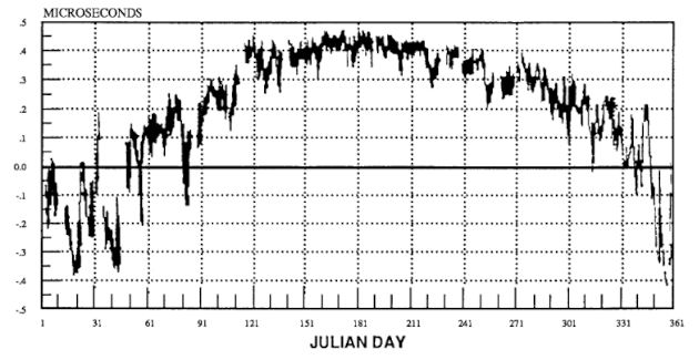
A pronounced seasonal effect is evident at this location. Xray TDs at this location are nearly 1 usec higher in the summer months than in December and January. Seasonal effects vary in magnitude with the season, chain, station pair, and the location of the observer. For example, there is almost no seasonal effect observed for this rate at Sandy Hook, NJ (Blizard and Slagle, 1987). The explanation for this phenomenon is that Sandy Hook is a LORMONSITE for the 9960 chain, and the monitor provides information that, among other purposes, is used to maintain a standard time difference at this location.
Diurnal (hourly within a day) variability is another form of temporal variability, as is illustrated in Figure 5 for the Xray secondary of the NEUS (9960) chain at Massena, NY. In this illustration, daily shifts in this TD of as much as 0,1 usec can be seen-smaller than the seasonal component at this location, but potentially significant nonetheless. As with seasonal variability, the magnitude of this effect varies with chain, station pair, and observer location.
Weather affects signal propagation, and the effects of the “Alberta Clipper” or “Siberian Express” (cold fronts with associated cold spells lasting from hours to days) sweeping across the Northeast can readily be detected in TD shifts as far south as South Carolina. In cold weather the speed of propagation of the signal is greater. Both temperature and humidity affect signal propagation.
The reader may ask the question:
“If seasonal, weatherrelated, anddiurnal factors can be quantified, why can’t thisinformation beused to reduce the overall uncertainty of the loran TDs?”
The answer to this astute question is that, in fact, it is possible to measure and quantify these factors, and (in principle) to broadcast a series of corrections to loran readings (similar to ASFs) foruse by themariner. Such a system, termed the difierential Loran-C system (DLCS), has been extensively studied (Blizard and Slagle, 1987) by the Coast Guard and proven to be feasible. Indeed, absolute accuracy of 30 meters or better in a local area has been demonstrated using differential Loran-C. However, DLCS has not been implemented to date. For most purposes (and in most locations), the accuracy of conventional loran is adequate, and any decision to increase this accuracy must be carefully evaluated on the basis of cost benefit calculations.
Factors Associated With Spatial Variability
Another groupof factors highlightedin Table 1 are those included under the rubric of factors that change from place to place, such as mountains, deserts, and structures. Although these factors are considered in the determination of the ASFs (see The Loran-C System: A More Detailed View“Understanding Loran Transmitters and Hyperbolic Systems”), not all the “microstructure” can be reflected in the estimated ASFs. To illustrate, near shore effects, bridges, powerlines, and other large structures (e. g. petroleum refineries, steel mills) affect loran signal propagation but are not accounted for in published ASFs. In extreme cases Loran-C TDs measured near such structures could result in navigational errors which exceed the absolute accuracy specifications. For example, the Verrazano-Narrows Bridge is a large suspension bridge arching over the entrance to New York Harbor.
When transiting between waypoints (see Practical Aspects of Loran Navigation“Mastering Loran-C Navigation: Techniques, Accuracy, Best Practices” for a discussion of waypoint navigation) in the centerline of the channel near this bridge, a calculation of the vessel’s position based upon Loran-C TDs may indicate that the vessel is several tens or even hundreds of yards outside the channel. The effect is greatest directly under the structure, and diminishes with distance. The distance where Loran-C TDs become unusable varies among structures, as does the amount of the TD shift. In Coast Guard trackline surveys (see: Radionavigation Bulletin, No. 11), it was noted that some powerlines affected Loran-C TDs as much as 500 yards distant, and caused distance errors up to 200 yards when directly under the powerlines. Although no method has yet been developed to predict and correct for these particular effects, the Coast Guard periodically identifies and publishes (Radionavigation Bulletin) a list of structures with the potential for adversely affecting the accuracy of loran navigation. Mariners are well advised to exercise caution when in the vicinity of these structures and not to rely solely on Loran-C for navigation in these areas.
Recallalsothat ASFs are less accurate within 10 NM of the coast (coast effect). For interesting data relative to this effect, see McCullough, et al, 1983. Although fixes determined by Loran-C may satisfy the 0,25 NM accuracy specification in these areas, such accuracy is not “guaranteed” for the system.
Other Factors
The accuracy with which loran LOPs are printed on charts is discussed in Loran-C Charts and Related Information“Loran-C Charts Key Components and Navigation Techniques”, and the accuracy of computer latitude/longitude conversions (imbedded into the Loran-C receiver logic) is discussed in Loran-C Receiver Features and Their Use“Understanding Loran Receivers: Features and Functionality”.
System Geometry
Perhaps the most important determinants of loran accuracy are those grouped under the classification of system geometry. Of particular relevance here are the crossing angles and the gradient of the Loran-C LOPs. These are discussed below, and in GDOP Explained and Illustrated“Understanding GDOP: The Key to Accurate GPS Positioning”, where the important concept of geometric dilution of position (GDOP) is explained and illustrated.
Geometric factors are among the most important determinants of Loran-C navigation accuracy. Geometric factors include the crossing angle and gradient, both of which vary throughout the coverage area.
Crossing Angles
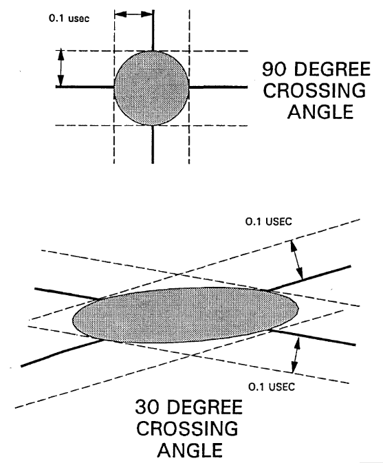
The crossing angle is the angle (more accurately the smallerof the two angles) between two LOPS that determine a fix. Most navigators are very familiar with the fact that the accuracy of a two-bearing fix varies with the crossing angle of the LOPS and that the optimal crossing angle for two LOPS is 90 degrees. The effects of large and small crossing angles are illustrated in Figure 6.

In this figure LOP 1 is assumed to be known without error, and LOP 2 to within an error shown by the dashed lines parallel to LOP 2. It is also assumed, for illustrative purposes, that the variability of LOP 2 is +/- 0,1 microseconds Recall (from the discussion in “The Loran-C System: A More Detailed View”) that either time or distance units may be used interchangeably.x. The best estimate of the observer’s position is where the two LOPs cross (denoted by the circle in Figure 5), but the possible (one dimensional) uncertainty in this position along LOP 1 depends not only on the uncertainty of LOP 2, but also on the crossing angle of the two LOPs. More specifically, the length of the interval of uncertainty is a function of the reciprocal of the trigonometric sin function of the crossing angle. As the inset graph in this figure shows, the length of this projection on LOP 1 is smallest at acrossing angle of 90 degrees and becomes very large for crossing angles of 30 degrees or less. Indeed, the length of the interval of uncertainty becomes – infinite for a zero degree crossing angle.
To illustrate, if the crossing angle were 90 degrees, the projection of the +/- 0,1 usec uncertainty in LOP 2 on LOP 1 would be O,1/(sin 90) =+/- 0,1 microseconds. However, if the crossing angle were as small as 15 degrees, the projection on LOP 1 would be 0,1/(sin 15) = nearly +/- 0,4 microseconds. Such small crossing angles are generally incompatible with the absolute accuracy specifications of the Loran-C system.
Other things being equal, the user should select those TDs with crossing angles closest to 90 degrees.
Figure 6 is simplified for illustrative purposes. In fact, there is uncertainty in both LOPs, not just one. In this more general case, the resulting uncertainty of the fix is not a one dimensional line, but rather a two dimensional area. Provided that the LOPs are at right angles, and the uncertainty in each LOP is the same (0,1 usec in this illustration), and that the possible errors in each TD are uncorrelated, this two dimensional area is a circle, as shown in Figure 7 (top).
In the top illustration (which satisfies the above assumptions) the vessel’s position would be known (in probabilistic terms) to be within the shaded circle of uncertainty. (The probability that the vessel would be in this area depends upon the probability content of each of the LOP bounds – more later.) However, assuming everything else were held constant but the crossing angle, the area of uncertainty would become distorted (into an ellipse) and very much larger if the crossing angle were decreased.
Figure 7 (bottom) shows how this circle is distorted and enlarged as the crossing angle is decreased from 90 degrees to 30 degrees. This distortion and enlargement becomes even more pronounced as the crossing angle is further decreased.
The crossing angle of Loran-C TDs can be shown (see Taylor 1961, Swanson 1978) to be related simply to the location of the vessel in the coverage area and to the location of the master and secondary stations. Figure 8 shows the geometry of the crossing angle for a loran Triad.
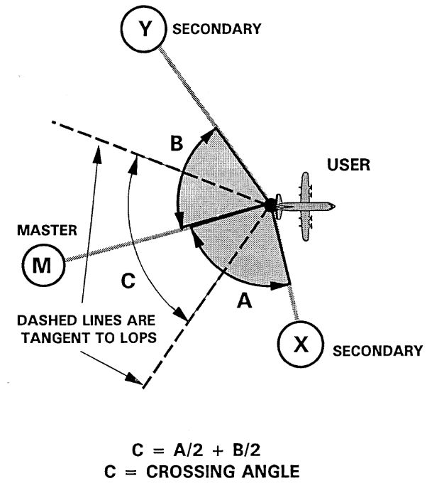
Specifically, if angle A is the angle between the great circles drawn from the user to the master and the Xray secondary, and angle B is similarly defined with respect to the master and the Yankee secondary, then the crossing angle (angle C in Figure 8 bounded by the dashed sector) is equal to A/2 + B/2. This follows from the so-called “optical” property of the hyperbola – the tangent to a hyperbola (i. e., to the LOP) at a point P bisects the angle between the lines joining P to the two foci of the hyperbola.
Figure 8 enables the reader to visualize how the crossing angle varies throughout the coverage area of the loran Triad. As drawn, the crossing angle is approximately 79 degrees. If the aircraft or vessel were to move in a “north-easterly” direction (north being the top of the page), the crossing angle would decrease, implying a less accurate fix. If the user were to move toward the master, the crossing angle would first increase and then decrease again, as the user draws close to the master. Remember that the crossing angle is the smaller of the two angles formed by the intersection of two LOPs. Crossing angles for positions along the baselines are not as close to 90 degrees as at certain interior points of the triangle formed by the master and two secondaries.
In practice, the crossing angles of the Loran-C LOPs are easy to measure from the loran overprinted chart, so that the determination of the secondaries with crossing angles nearest to 90 degrees at any position on the chart, is likewise easy.
Gradient
The gradient is calculated as the ratio of the spacing between adjacent loran TDs (measured in ft, yards, nautical miles) and the number of microseconds difference between these adjacent LOPs Technically,the gradient is defined as the rate of change of distance with respect to TD, i. e., is the derivative of this function. It is calculated from charts in terms of numerical differences. Some authors use the word “lane” interchangeably with gradient.x. Most commonly, the gradient is expressed as ft/usec or meters/usec. Figure 9 illustrates the computation of gradients for two hypothetical sets of loran LOPs such as would be found on a loran overprinted chart. In the illustration at the top of this figure, loran LOPs are spaced 10 usec apart (i. e., 25 850 – 25 840) and 4 nautical miles apart.
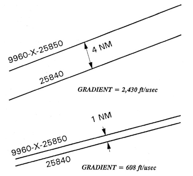
The gradient in this case would be 4(6,076)/10 = 2,430 ft/usec. In the bottom illustration, this gradient is 608 ft/usec. If it is assumed that there is aconstant error of the TD (as measured in usec) throughout the coverage area, it follows that (other factors held constant) loran LOPs with smaller gradients will result in a fix with greater accuracy. Note that computation of the gradient of a given rate at a given location is a simple task of measuring the distance (in nautical miles or other convenient units) between adjacent Loran-C TDs as printed on the appropriate chart and dividing this distance by the spacing (in usec) between the LOPs.
As with crossing angles, gradients vary throughout the coverage area. Figure 10 shows how the gradient of a single TD varies with location for the example originally given in The Loran-C System: A More Detailed View“Understanding Loran Transmitters and Hyperbolic Systems”. As can be seen, the gradient is smallest in the vicinity of the baseline (e. g., point “A” in Figure 10). Infact, the gradient is constant anywhere alone the baseline and numerically equal to 491,62 ft/usec. It can also be shown that if the gradient exceeds 2 000 ft/usec, the 0,25 NM absolute accuracy requirement for Loran-C system accuracy will not be satisfied.
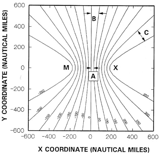
Note from Figure 10 that the gradient grows larger as you move away from the baseline, from point “A” to point “B.” The increase in gradient with increases in distance from the baseline is not constant – increases are very much larger in the vicinity of the baseline extension. Note that the gradient at point “C” in Figure 10 is even larger than at “B“. Had other LOPs been shown in Figure 10 even closer to the baseline, the increase in gradient would have been more dramatic. This is one of the major reasons why it is not recommended to use secondaries in the vicinity of their baseline extensions Recall from the discussion in the beginning of this chapter that ambiguous positions are associated with baseline extensions.x. Users at or near position “C” in Figure 10 would be well advised to select another secondary – in lieu of the Xray secondary – for more accurate navigation.
Small gradients are associated with most accurate fixes. For a given master-secondary pair, gradients are smallest near the baseline. Gradients are very large in the vicinity of a baseline extension. Other things being equal, the user should select those TDs with the smallest gradients.
The explosive expansion of the gradient near the baseline extension is the reason why secondary stations should not be used in the vicinity of the baseline extensions, and why these lines are shown on nautical charts. Important areas of baseline extension in the United States include the area east of the Xray secondary of the NEUS chain located on Nantucket, MA, the area south of the Yankee secondary in Carolina Beach NC for this same chain, the area southeast of the Yankee secondary of the SEUS (7980) chain, located in Jupiter, FL, etc. These areas can be clearly seen from inspection of the coverage diagrams presented in Introduction and Overview of Loran-C“Data Sheets and Coverage Diagrams”.
Brief Remarks on Station Placement
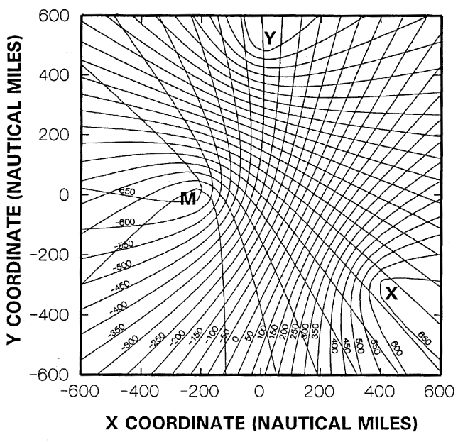
Careful examination of Figure 10 suggests that the gradients in a loran coverage area could be reduced and the crossing angles improved if the master and Xray secondary were placed a greater distance apart. This conjecture is, indeed, correct. Long baseline lengths serve to increase the accuracy of loran fixes in the coverage area. This is a well-known principle in the design of loran chains. Other things being equal, the fix accuracy of the Triad shown in Figure 2 would improve if either of the baseline lengths were extended. As well, the crossing angles of many of the LOPs would improve if the two baselines were more nearly at right angles. Figure 11 shows the LOPs that would result if the Xray secondary were relocated on the original grid from (200, 0) to (400, -300) – that is if the crossing angle of the two baselines were changed to 94 degrees (86 degrees, when subtracted from 180) rather than the 70 degrees in the original Triad, and the length of the Xray secondary were lengthened to 671 miles from the original 400 miles.
In this illustration the spacing of the Xray LOPs is still 50 miles (or its equivalent in TD units), and the TD spacing of the Yankee LOPs is likewise unaltered. But note how the crossing angles have improved throughout the “northeast” part of the coverage area (compare Figures 2 and 11), as have the gradients. Although the lattice is still obviously distorted, it is much more nearly rectangular than the original. This chain configuration is decided by superior to that assumed initially. From a geometric perspective alone, further lengthening of either baseline would help, as well as shifting the angle between the two baselines. Incidentally, Figure 11 shows clearly the position ambiguities in the vicinities of the baseline extensions of the two master-secondary pairs.
However, there are practical limits that need to be considered in selecting locations for loran stations. First, there are numerous physical and political constraints which limit the placement of these stations. These stations need to be located on land, and in friendly or cooperating countries. Physical and political constraintslimit baseline lengths and crossing angles. Second, there are technical constraints which also impose limits on the length of baselines. The selection of long baseline lengths to obtain high accuracy often is not compatible with optimum coverage area because distance limitations on signal propagation prevent simultaneous reception of signals from the most distant stations. Of course, the useable baseline distance can be increased by increasing the transmitter power, but a diminishing returns situation prevails – substantial power increases are required as the master and secondary stations are located farther apart.
Putting it Together: drms
The advice to select secondaries with 90 degree crossing angles and small gradients is fundamentally sound, but occasionally there is a tension between these objectives Asnoted, gradients of individual rates are smallest near their respective baselines, while optimal crossing angles are found in interior points. Moreover, the gradients of both sets of LOPs need to be considered. Unless some aggregate measure of accuracy is at hand, it is not obvious how to make tradeoffs among these measures so as to maximize fix accuracy. Use of the 2 drms accuracy measure resolves these difficulties.x. Therefore, it is very useful to have an accuracy measure which includes the effects of both these geometric variables. Although several such measures can be defined, the quantity “2 drms” is most commonly used. This quantity, 2 drms, is the radius of a circle about the vessel’s apparent position such that, in at least 95 % of the fixes, the vessel’s actual position would be located somewhere within this circle.
Mathematically, 2 drms is given by the equation:
where:
- A, B, C – angles defined in Figure 8;
- ρ – correlation coefficient between the measured TDs, generally taken to be 0,5 for purposes of calculation;
- K – baseline gradient, 491,62 ft/usec, and;
- σ – common value of the standard deviation of each TD, generally taken to be 0,1 usec for 2 drms absolute accuracy calculations.
The Loran-C accuracy specification is expressed in terms of 2 drms; 2 drms plus ASF error must be less than or equal to 0,25 NM throughout the coverage area. Indeed, the accuracy limits on the range of coverage of loran triads (and, derivatively, loran chains) are determined as the largest range such that 2 drms is less than or equal to 0,25 NM throughout the coverage area.
Equation (1) can be used to calculate how accuracy varies throughout the coverage area. The various terms in this equation identify the key parameters and variables affecting the 2 drms accuracy measure. Figure 12 shows these schematically. In broad terms, there are three sets of variables that determine 2 drms. These include the statistical characteristics of the transmitted signal, the locations of the transmitters, and the position of the user. Key statistical parameters include the standard deviation of the TDs (generally taken as 0,1 usec for each TD), and the correlation coefficient between the measured TDs (which varies throughout the coverage area, but often set equal to 0,5 for calculation of 2 drms).
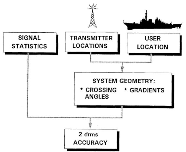
The transmitter locations and the user’s position determine the angles A, B, and C shown in Figure 8. The location of the transmitters and that of the user jointly determine the crossing angles and gradients referred to earlier. Collectively, all these factors determine 2 drms. The user has no control over the signal characteristics of the Loran-C transmissions, nor the locations of the transmitters. However, for many locations, the user does have a choice among chains, and secondaries within these chains. In portions of the eastern United States, for example, the user can choose among three chains. West Coast users are less fortunate. For best results, the user should select the secondaries so as to minimize 2 drms, or equivalently, to maximize the accuracy of any fixes. This choice is described below.
Accuracy vs. Location in the Coverage Area
From the point of view of the user, the significance of the above equation is that the absolute accuracy of fixes derived from any two station pairs can be calculated, and the “best” station pairs can be selected from among the available alternatives. Although these calculations are not conceptually difficult, a computer is required for rapid and numerically accurate solution. In any event, it would be very tedious if the user had to make these calculations for each station pair of each chain in order to select the best station pairs – particularly as these calculations would have to be replicated for every possible position in the coverage area.
The quantity 2 drms is the radius of a circle within which 95 % of the possible fixes lie. Secondaries should be selected to minimize the value 2 drms for most accurate.
Fortunately, these calculations have already been made, and are given in Introduction and Overview of Loran-C“Data Sheets and Coverage Diagrams”. Figure 13 (taken from COMDINST M16562.4, Specification of the Transmitted Loran-C Signal), shows results of these calculations for the various station pairs in the NEUS (9960) chain. For example, diagram “C” in Figure 13 shows accuracy contours for the master-Xray and master-Yankee station pairs. The solid line in this diagram shows the 2 drms contour of 1 500 ft. absolute accuracy, the dashed line 1 000 ft., and the dotted line 500 ft. Imagine, for example, that a vessel were located off Cape May, NJ. As can be seen, this location is well within the limits of the 500 ft. 2 drms contour, indicating that the absolute accuracy of the Loran-C system using these master-secondary pairs is quite high, and significantly better than the 0,25 NM absolute accuracy specification. Note from this illustration that these contours are well clear of the baseline extensions south of the Yankee secondary, or east of the Xray secondary.
Similarly, diagram “B” in Figure 13 shows the same information for the master-Whiskey and master-Xray station pairs. These station pairs provide accurate coverage north of Massachusetts, but offer accuracy little better than 1 500 ft in the area off Cape May, NJ. A careful examination of all the diagrams within Figure 13 indicates that the master-Xray and master-Yankee station pairs provide the most accurate Loran-C coverage over a broad ocean area stretching southward from Nantucket, MA, to the Yankee secondary in North Carolina. Therefore, a mariner using the NEUS (9960) chain anywhere within this area should select these secondaries for navigation.
Coverage Diagrams
The range limits of the coverage diagram are selected to ensure that the absolute accuracy of a Loran-C fix (expressed as 2 drms) is at least 0,25 NM.
However, potential fix accuracy is only one criterion used in the determination of the coverage area of each Loran-C chain. It is also important to have reliable Loran-C reception. The Loran-C receiver has to be able to acquire and track a transmitted signal imbedded in “noise.” This noise arises principally from atmospheric sources (noted above),and typically has a strength which exceeds that of the signal. The key measure of the relation between the signal strength and that of the noise is the signal-to-noise ratio (SNR). It is expressed as a ratio of the average signal strength to the root mean square noise strength Fornoise estimation purposes, the upper 95 % one-sided confidence limit is used as averaged over each 4-hour period of the day, for each season of the year. This computation is made for a selected point in the middle of the coverage area.x. The loran receiver’s tasks of acquiring and tracking the signal are reliably accomplished when the SNR is high, but become more difficult as the SNR is lowered, and virtually impossible beneath a critical value. (The critical value varies among receivers.)
Signal strength as measured at a receiver location depends upon the transmitter power, antenna type, conductivity of the mixed land sea path over which the ground wave travels, and upon the range from the transmitter to the observer. In particular, the signal is attenuated as it travels from the transmitter to the receiver; the signal strength decreases as rangeincreases. The strength of the noise is a function of many factors, but is typically dominated by atmospheric noise.
Mathematical models have been developed to calculate signal attenuation as a function of the distance from a loran transmitter, as well as to estimate noise. Using these models (typically imbedded in computer routines) it is possible to estimate the SNR of a signal as a function of range from the master station and associated secondaries in the loran chain. For range planning: Dumoses. it is assumed that the loran receiver requires a SNR of 1/3 or greater to provide reliable reception. In fact this SNR limit is conservative, many loran receivers can track signals adequately with SNRs of 1/10 or even less. Therefore, it is possible to calculate the range limit for each set of station pairs in the loran chain.
Figure 14 displays the results of an illustrative set of SNR calculations. This illustration shows the variation of SNR (from 0 to a maximum of 5) with range (in hundreds of nautical miles) for signals of various power (275 kW and 800 kW, representative of a secondary and master station power respectively) in two noise environments. The “average noise” environment (200 uv/meter) is representative of good weather conditions, and the “high noise” value (800 uv/meter) is typical of what might be expectedduring a thunderstorm. (Other assumptions in this calculation are summarized in Culver, 1987 and relate to “fair soil” ground path.
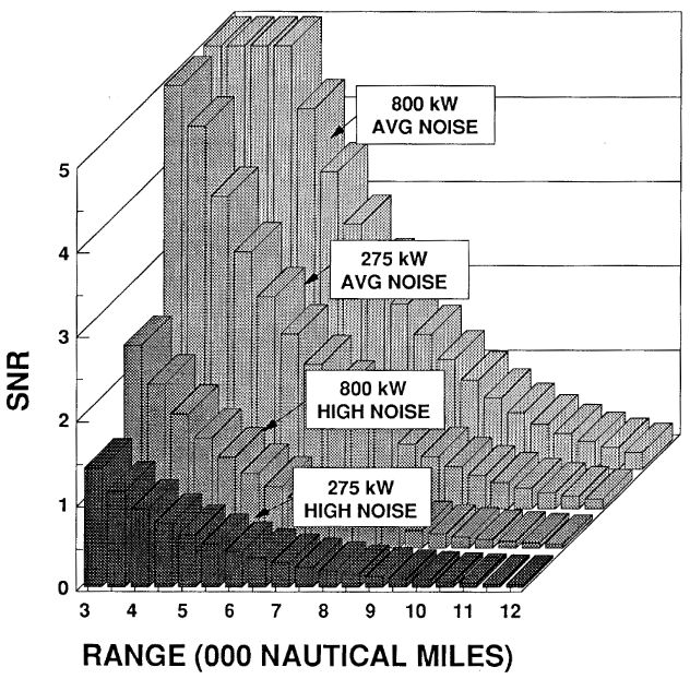
This is one of the simpler models from among several that can be used for SNR calculations.) Note from Figure 14 that the SNR decreases with distance, and that the SNR at the receiver is dependent upon the distance from the transmitter, the power of the transmitter, and the atmospheric noise level. For any combination of transmitter power and noise, the range at which the SNR falls beneath the assumed limit of 1/3 (0,333) can be calculated. In this set of calculations, this range limit varies between approximately 600 and 1 100 miles, depending upon the transmitter power and the atmospheric noise level. Other things being equal, a doubling of the transmitter power results in only a 41 % increase in the SNR, apoint that underscores the practical difficulties of increasing the baseline lengths by increasing the transmitter power.
Remember also that each station in the Triad in use must be received with a minimum SNR for acceptable navigation, so the range coverage limit is calculated based upon the signals from the master and both secondaries.
The maximum range of the Loran-C system is defined as that range which satisfies both accuracy and SNR criteria. This is the limit of coverage shown in the Loran-C coverage diagrams. Adequate Loran-C navigation may be possible at ranges exceeding this maximum range (operationin so-called “fringe areas“), but adequate reception of a navigationally accurate signal is assured within the published coverage limits of the system.
Chain Selection
As noted, many loran receivers will automatically select both the loran chain and secondaries for use. As receiver design has advanced, these selection algorithms have become quite sophisticated, at least for some makes and models of receiver. However, the criteria used for automatic selection of chains and secondaries may be inappropriate in some instances. For example, some earlier loran receivers selected secondaries principally on the basis of the SNR. Although signal strength is certainly relevant to the selection of secondaries, it is not the only appropriate criterion. Moreover, there are circumstances where selection of the strongest signals would be contraindicated. (See Doyle, 1990, for an example relevant to the West Coast chain.)
All Loran-C receivers have the capability for manual chain and secondary selection, and users shouldknow how to select these chains and secondaries for optimal reception. Table 2 provides three useful criteria for selection of the appropriate chain and secondaries. Assuming that there are no scheduled outages, and that one chain can be used for the entire voyage route, these criteria reduce to selection of the optimal secondaries shown in the coverage diagrams (e. g., Figure The Loran-C System: A More Detailed View“An actual Loran-C chain showing transmitter and monitor locations for the NEUS chain (GRI 9960)”).
| Table 2. Chain selection criteria These criteria apply when manually selecting a Loran-C chain. Commercial receivers use a variety of criteria for automatic chain selection.x | |
|---|---|
| Criterion | Brief Description |
| Route/Destination Coverage | Whenever possible, select a chain that can be used throughout the entire voyage. This allows you to “lock on” your receiver prior to departure and maintain track throughout the trip without having to change chains. |
| Adequacy of Secondary Stations | Chain selection also depends upon the associated secondary stations. Select a chain that includes secondaries having the greatest potential for accurate navigation. |
| Availability of Service | Avoid using chains that have scheduled outages during the period of the planned voyage. Scheduled outages are published in the Local Notices to Mariners, and Notices to Airmen, and announced on Coast Guard radio broadcast. Obviously unscheduled outages are also relevant to chain selection, but these are infrequent and (by definition) cannot be anticipated in prevoyage planning.x |
Practical Pointers
Practical Aspects of Loran Navigation“Mastering Loran-C Navigation: Techniques, Accuracy, Best Practices” presents practical pointers on the use of loran. However, it is useful to consider the practical implications of the above discussion of system accuracy. At the most basic level, no navigation system should be used without aclear understanding of its limitations. Some of the key limitations for Loran-C are those on system absolute and repeatable accuracy. Unless the user has completed a survey (however informal) and determined actual TDs for important locations (e. g., entrance buoys, channel centerlines, channel turnpoints, rocks, shoals, and other obstructions to safe passage) or has access to such survey data, passages should be planned to keep the vessel well clear (considering the absolute accuracy of the system) of potential hazards to navigation. As well, the navigator should remember that loran accuracy is degraded (possibly beneath the stated 0,25 NM accuracy) in areas within 10 NM of shore and, in any event, when in close proximity of bridges, powerlines, and other large structures.
The mariner should also pay close attention to the selection of chains and secondaries to use, so as to maximize the absolute accuracy of the system. Receivers may select stations based on other criteria (e. g., SNR) that, while relevant, are not directly related to system accuracy. The loran user should not passively accept the “default” selection criteria of the receiver, without at least noting which secondaries are chosen and manually overriding the automatic selection when appropriate.
Users should try, whenever possible, to exploit the repeatable accuracy of the system, by deliberately recording locations of interest and navigational relevance. Each voyage presents the opportunity to record the TDs of navigationally relevant locations, and to check the repeatable accuracy of the system, including the receiver, by other methods (e. g., horizontal sextant angles, buoys, etc.). These activities can be integrated into a recreational voyage without consuming undue amounts of time. Cumulatively over several voyages, a very useful “personal data bank” of information can be developed. The utility of this information will be apparent on the first occasion that weather deteriorates to such a degree that a true “instrument approach” is needed to return safely to home port.
Incidentally, TDs of navigationally relevant locations can be stored in the Loran-C receivers (as waypoints), but should also be recorded in a separate hard-copy log. The utility of a written record is not only because receivers may not be able to store enough waypoints, but also because electronically stored waypoints can be accidentally erased.
Finally, it is worth repeating here that no one system of position fixing should be used exclusively. The prudent mariner or aviator is one who appreciatesboth the capabilities and limitations of the system, and uses all relevant information (e. g., DR plots, soundings, visual observations, radar, etc.) for navigation.
No one system of position fixing should be used exclusively. The prudent mariner uses all available information (e. g. soundings, visual observations, of landmarks, fixed and floating ATONs, radar) for navigation.

- Abramowitz, M., et al. “Approximate Method for RapidLoran Computation,” Navigation; Journal of the Institute of Navigation, Vol. 4, No. 1, March 1954, pp. 24-27.
- Alexander, G. “The Premier Racing Tool,” Ocean Navigator, Issue No. 20, Jul/Aug 1988, pp. 37, er seq.
- Anonymous. “Loran: Installation Pitfalls, and How Friendly Should Your Loran Be?” Practical Sailor, Vol. 11, No. 24, December 15, 1985, pp. 1, et seq.
- Anonymous. Manual on Radio Aids to Navigation, International Associationof Lighthouse Authorities, Nouvelle Adresse, 13 Rue Yvon-Villarceau 75 116, Paris, 1979.
- Appleyard, S. F. Marine Electronic Navigation. Routledge and Kegan Paul Ltd., Boston, MA, 02108, 1980.
- Ashwell, G. E., B. G. Pressey, and C. S. Fowler. The Measurement of the Phase Velocity of Ground Wave Propagation at low Frequencies Over a Land Path. Proceedings of the Institute of Electrical Engineering (London) 100 Part III, 1953.
- Bedford Institute of Oceanography. Loran-C Receiver Performance Tests, Bedford Institute of Oceanography, P. O. Box 1006, Dartmouth, NovaScotia, Canada, B2Y 4A2.
- Blizard, M. M. et al. Harbor Monitor System Final Report, CG-D-17-87, ADA 183 477, Dec. 1986, Available through the National Technical Information Service, Springfield, VA, 22161.
- Blizard, M. M., Lt. and CWO 3 D. C. Slagle. Differential Loran-C System Final litter, Draft, United States Coast Guard, January 1987.
- Blizard, M. M. and D. C. Slagle, “Loran-C West Coast Stability Study,” Proceedings of the Fourteenth Wild Goose Technical Symposium, Wild Goose Association, Bedford, MA, 1985.
- Brogdon, B., “Loran Expansion,” Ocean Navigator, Issue No. 42, SeptfOct 1991, pp. 87, et seq.
- Brogdon, W. “Loran Hook, a Little Known, Foible Explained,” Boating, August 1991, p.42.
- Brogdon, W. “Electronic Errors,” Ocean Navigator, Issue No. 40, June 1991,pp. 70, etseq.
- Brogdon, W. “Pathfinders,” American Hunter, Vol. 19, No. 7, July 1991.
- Burt, W. A., et al. Mathematical Considerations Pertaining to the Accuracy of Position, Location, and Navigation Systems, Part I, Stanford Research Institute, 1966. Available from National Technical Information Service, AD-629609, US Department of Commerce, 5825 Port Royal Road, Springfield, VA 2215 1.
- Canadian Coast Guard, Aids and Waterways Branch. A Primer on Loran-C, Ottowa, Ontario, Canada, 1981.
- Connes, K. The Loran, GPS & NAVICOMM Guide, Butterfield Press, 1990.
- Culver, C. “A New High Performance Loran Receiver,” Proceedings of the Sixteenth Annual Technical Symposium, The Wild Goose Association, 20-27 October 1987, pp. 282, et seq.
- Dahl, B. “Adopting Loran-C to Everyday Navigation,” Cruising World,May 1983,pp. 40-45.