Delve into the intricacies of Loran transmitters and hyperbolic systems in this comprehensive article. Discover key concepts such as signal characteristics, chain configurations, and the principles of phase coding.
- Introduction
- Loran Transmitters, Chains, and Some Basic Definitions
- Signal Characteristics and Some Important Definitions
- Chain Configuration
- Other Definitions
- Hyperbolic Systems: A Second Look
- Hyperbolic Geometry On a Plane
- Equivalence Between Distance and Time
- More Exact Calculations
- Primary Phase Factor (PF)
- Secondary Phase Factor
- Additional Secondary Phase Factor (ASF)
- ASF Tables
- Use of Tables
- Groundwave versus Skywave Propagation
- Pulse Architecture and Related Technical Matters
- Phase Coding
- Blink Coding
- Concluding Comments
Understand the differences between groundwave and skywave propagation, and explore practical applications of these technologies in navigation and communication. Enhance your knowledge of radio signal systems and their significance in today’s tech landscape.
Introduction
This article provides a more detailed exposition of the Loran-C system. In particular, a more technical presentation of the logic of hyperbolic systems is given, along with additional details on chains, signal propagation, ASF corrections, chain coverage, and salient characteristics of the transmitted signal. Loran-C Position Determination and Accuracy“LORAN-C System: Accuracy and Position Determination” extends this discussion to loran accuracy and its determinants, and methods for plotting positions.
Loran Transmitters, Chains, and Some Basic Definitions
As noted in Introduction and Overview of Loran-C“What is Loran-C? Exploring Its Role in Marine Radionavigation”, a basic element of the Loran-C system is the loran chain. This chain consists of three or more stations (generally abbreviated LORSTAs for loran stations) , including a master and at least two secondary transmitters. Each master-secondary pair enables determination of one LOP, and two LOPS are required to determine a position. Each Loran-C chain provides signals suitable for accurate navigation over a designated geographic area termed a coverage area. The limits of each chain’s coverage area are given in Introduction and Overview of Loran-C“Data Sheets and Coverage Diagrams”, and discussed in conceptual terms in this chapter and in Loran-C Position Determination and Accuracy“LORAN-C System: Accuracy and Position Determination”.
The coverage areas of the various Loran-C chains overlap somewhat, and there are many areas in the United States and nearby coastal waters where two (or more) chains can be received and used for navigation For reasons that will be apparent in “Loran-C Position Determination and Accuracy”, overlapping coverage areas are desirable. Redundant coverage not only increases the likelihood that the user can receive critical navigation information, but also offers the possibility of increased fix accuracy.x. Criteria for selection of the most appropriate chain for navigation in areas covered by more than one chain are discussed in Loran-C Position Determination and Accuracy“LORAN-C System: Accuracy and Position Determination”.
Table 1 identifies the ten Loran-C chains that provide coverage of the United States and contiguous areas, along with their common abbreviations, GRI designators (defined and discussed below), and the year that each chain was first completed.
| Table 1. Loran-C chains providing coverage of the United States and contiguous areas | |||
|---|---|---|---|
| Chain Relevant data on each of these chains, including the location of the master and secondary stations and the coverage diagram for the chain, can be found in “Data Sheets and Coverage Diagrams”.x | Common Abbreviation | GRI Group repetition interval designator, discussed later in this chapter.x Designator | Year Completed Portions of the chain may have been completed earlier. The date given in this table is the first year that the entire chain was operational.x |
| North Pacific Chain | NORPAC | 9990 | 1981 |
| Gulf of Alaska Chain | GOA | 7960 | 1977 |
| Canadian West Coast Chain | CWC | 5990 | 1980 |
| US West Coast Chain | USWC | 9940 | 1977 |
| North Central US Chain | NOCUS | 8290 | 1991 |
| South Central US Chain | SOCUS | 9610 | 1991 |
| Great Lakes Chain | GL | 8970 | 1980 |
| South East US Chain | SEUS | 7980 | 1979 |
| North East US Chain | NEUS | 9960 | 1979 |
| Canadian East Coast Chain | CEC | 5930 | 1983 |
Closure of the so-called midcontinent gap This was an area of the United States where Loran-C coverage was missing. Closure of this gap benefits mariners who boat in the central states, but is of particular interest to aviation and terrestrial users of the Loran-C system.x was completed with the commissioning of the NOCUS and SOCUS chains in 1991-an event marked with much pageantry as a sort of navigational equivalent of the completion of transcontinental railway of yesteryear.
Loran-C transmitters vary in radiated power from less than 200 kW (kilowatts) to over 2 MW (megawatts). To lend some perspective, the radiated power output of a typical AM station in the United States might be 5 kW. For FM transmissions the typical output would be larger, say 50 kW. Exact comparisons of power output are difficult to make, because the loran transmits only pulses. Nonetheless, in semi-quantitative terms at least, loran transmitters are quite powerful. Among other factors, the radiated power controls the range at which a usable signal can be received and, therefore, the coverage area of the chain.
Some transmitters have only one function (i. e., to serve as a master or secondary in a particular chain), but many transmitters are “dual rated,” meaning that these can serve one function in one chain, and yet another in a neighboring chain. For example, the Dana, IN, transmitter serves as the Zulu secondary in the NEUS (9960) chain, and also as the master transmitter for the Great Lakes (8970) chain. Dual rating is desirable because, other things being equal, land acquisition costs and siting difficulties are reduced.
Signal Characteristics and Some Important Definitions
Characteristics of the transmitted Loran-C signal are discussed in some detail below, but briefly, the transmitted signal consists of a series or group of pulses (each of a defined waveform discussed later). For the master signal, a series of nine pulses are transmitted (eight spaced 1 000 usec apart, followed by a ninth 2 000 usec later). Pulsed transmission reduces the power requirements for system operation, assists signal identification, and enables precise timing of the signals. Secondaries transmit a series of only eight pulses, each spaced 1 000 usec apart. This difference in the number of pulses, among other properties of the signal, enables some loran receivers to distinguish the signals from the master from those of the secondary stations. Most receivers use phase codes, discussed below, for this purpose, however.
The master and each secondary in the chain transmit in a specified and precisely timed sequence. First, the master station transmits. Then, after an interval sufficientto allow the master signal to propagate throughout the coverage area, the first secondary in sequence transmit This scheme ensures that the first signal received by an observer in the coverage area is from the master. Reception of the master “starts the clock” in the loran receiver to measure the time difference.x, and so forth. Normally, the secondary stations transmit in the alphabetical order of their letter designator – e. g., Whiskey before Xray before Yankee, etc.
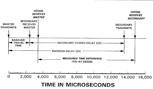
The secondary transmission is timed as follows: after the master signal reaches the next secondary in sequence, this secondary waits an interval, termed the secondary coding delay (SCD) or simply coding delay (CD), to transmit. The total elapsed time from the master transmission until the secondary transmission is termed the emission delay (ED). The ED is equal to the sum of the time for the master signal to travel to the secondary (termed the baseline travel time or baseline length (BLL)) and the CD. Next, other secondaries (each with a specified CD/ED) transmit in sequence. The sequence is completed when the master again transmits the nine pulse group.
The length of time between successive transmissions of the master’s pulse groups is termed the group repetition interval (GRI), and is expressed in microseconds (usec). The GRI designator is the GRI divided by ten, and is used as a symbol to identify anddesignate the loran chain The terms GRI and GRI designator are often used interchangeably-it is clear from the number of digits which term is being referred to. GRIs are five-digit numbers, GRI designators are four-digit numbers.x. Thus, the interval between successive transmissions (GRI) of the master pulse group for the Northeast US (NEUS) chain is 99 600 usec (about 0,1 sec), so the GRI designator for this chain is 9960. The GRI is chosen for each chain to be sufficiently large so that the signals from the master and each secondary in the chain have sufficient time to propagate throughout the chain’s coverage area before the next cycle of pulsed transmissions begin Setting a GRI for a chain involves the consideration of several factors. On the one hand, signal-to-noise considerations argue for relatively small GRIs. The Group Repetition Rate (reciprocal of the GRI) will be largest for short GRIs, and the increased duty cycle will provide an improvement in the ratio of signal-to-noise.On the other hand, the pulse spacing,receiver recovery time, necessity for coding delays, baseline lengths, the distances between secondaries, and the number of secondaries impose constraints that collectively argue for longer GRIs. As with many technical parameters of the Loran-C system, practical compromises and trade offs need to be made. In the end, however, these considerations are of much greater relevance to the system designer than to the user.x.
Continuing the example of the NEUS (9960) chain, the CDs and BLLs for the various secondary stations in this chain are:
- Whiskey (CD 11 000 usec/BLL 2 797,20 usec);
- Xray (CD 25 000 usec/BLL 1 969,93 usec);
- Yankee (CD 39 000 usec/BLL 3 221,64 usec);
- Zulu (CD 54 000 usec/BLL 3 162,06 usec).
This information is essential for computation of theoretical time differences (TDs) or loran LOPS, as illustrated below.
As apoint of interest, dual-rated stations are periodically faced with an impossible task of radiating two overlapping pulse groups at the same (or nearly the same) time. To resolve this difficulty, one of the signals is blanked or suppressed during this time period. Priority blanking occurs when the same signal is always blanked, whereas alternate blanking occurs when blanking alternates between the two rates. The type of blanking used for dual-rated stations is shown in the data sheets given in Introduction and Overview of Loran-C“Data Sheets and Coverage Diagrams”.
The stations in the loran chain transmit in a fixed sequence which ensures that TDs can be measured throughout the coverage area. The length of time in usec over which this sequence of transmissions from the master and the secondaries takes place is termed the Group Repetition Interval (GRI) of the chain.
All Loran-C chains operate on the same frequency (100 kHz), but are distinguished by the GRI of the pulsed transmissions. GRIs for each chain, together with CDs and EDs for each secondary in the chain are also given in Introduction and Overview of Loran-C“Data Sheets and Coverage Diagrams”.
Chain Configuration
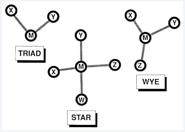
The physical locations of the master and secondary transmitters (among other factors) is an important determinant of both the accuracy and coverage area of the Loran-C chain. Although the configuration (site pattern of the transmitters) of each loran chain differs, it is convenient to group these configurations into three generic categories; the Triad (master and two secondaries), the Wye (master and three secondaries in a spatial arrangement roughly resembling the letter “Y“), and the Star (master and four or more secondaries roughly resembling a star in appearance), as illustrated in Figure 1. For example, the Icelandic (9980) and Labrador (7930) chains are illustrations of Triads, the North Pacific (9990) is a Wye, and the NEUS (9960) is in a Star configuration.
Loran-C chains
These generic configuration categories are only approximate descriptions – the NEUS (9960) chain, for example, would be classified as a star in this taxonomy but, as can be seen from Figure 2 This figure also contains a great deal of other useful information. This figure is referred to later in the chapter, and again in “The Loran-C System: A More Detailed View”.x, the resemblance is not literal. Interestingly enough, each transmitter in the 9960 chain is dual rated; the Zulu secondary is discussed above, the master, located in Seneca, NY, also serves as the Xray secondary for the Great Lakes (8970) chain, the Yankee secondary , located in Carolina Beach, NC, also serves 9s the Zulu secondary for the SEUS (7980) chain, the Xray secondary, located in Nantucket, MA, also serves as Xray secondary for the Canadian East Coast (5930) chain, and finally, The coverage area (discussed in Loran-C Position Determination and Accuracy“LORAN-C System: Accuracy and Position Determination”) the Whiskey secondary, located in Caribou, ME, for the NEUS (9960) chain is also shown in also serves as the master station for the Canadian Figure 2 enclosed by the long dashedlines. In East Coast (5930) chain.
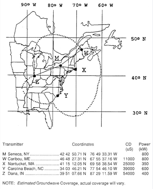
The coverage area (discussed in Loran-C Position Determination and Accuracy“LORAN-C System: Accuracy and Position Determination”) for the NEUS (9960) chain is also shown in the Figure 2 enclosed by the long dashed lines. In this chain the dimensions of the coverage area are each nearly 1 000 NM in length – an area several hundred thousand square miles in extent. Off-shore coverage extends several hundred miles.
Other Definitions
The geographic line (technically the arc segment of the great circle) connecting the master and each secondary is termed the baseline for the master-secondary pair. The length of the baseline (in nautical miles) varies with the chain and the individual master-secondary pair, but is typically several hundred miles. Other points on this same great circle containing the baseline (i. e., on the extension of the baseline beyond the two stationsjoined) are part of what is termed the baseline extension.
Key technical terms defined in this section include GRI, ED, CD, baseline, baseline travel time, and baseline extension.
As noted below, navigational use of a particular master-secondary pair in the area of the baseline extension is problematic. Baseline extensions are shown on nautical charts, as discussed in Loran-C Charts and Related Information“Loran-C Charts Key Components and Navigation Techniques”.
Hyperbolic Systems: A Second Look
As noted in Introduction and Overview of Loran-C“What is Loran-C? Exploring Its Role in Marine Radionavigation”, hyperbolic navigation systems function by measuring the time differences in reception of signals from the master and secondary transmitters.This chapter expands upon the basic idea of the hyperbolic system – with particularemphasis on the Loran-C system. This section is fairly technical, and may be skipped by the reader uninterested in such detail. Overall, the key technical points are simple enough.
First, the locus of points of constant difference in distance from two stations is described by a mathematical function termed a hyperbola. Second, the same is true for time differences (assuming a constant propagation velocity). Therefore, LOPS of constant TDs are likewise hyperbolas. Finally, the real world is slightly more complex than the assumption of a constant propagation velocity would indicate. Precise calculations of the physical location of loran LOPS require a series of correction factors to be applied to account for the fact that loran waves slow down over seawater or land (compared to propagation through the atmosphere).
Hyperbolic Geometry On a Plane
To be concrete, suppose that (as some ancients did) the earth were a flat plane, defined by the usual rectangular (X, Y) coordinate system, where the units of the X and Y axis areinnautical miles from an origin located at the point (0, 0). Now suppose that two loran stations are located on this lattice, a master station located at the point M = (xm, ym) = (-200, 0) along the X axis, and an Xray secondary station at the point S = (xs, ys) (200, 0) – some 400 NM to the right along the X axis. Consider an arbitrary point A = (xa, ya) on the lattice. From elementary plane geometry, the distance (in nautical miles) from point A to the master M, denoted dam, is:
or, in terms of the defined location of the master station, equation (1) reduces to:
Likewise, the distance from point A to the secondary, denoted das, is given by:
Finally, the difference between these distances, denoted Z, is given by:
Figure 3 shows how this distance difference function, Z, varies with the location of the point A in the plane. This figure is truncated at Z = -350 (point A 350 miles chosen to the master than to the secondary) and at Z = 350 (point A 350 miles chosen to the secondary than to the master).
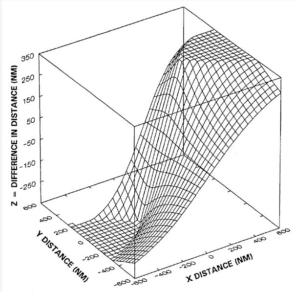
A more typical presentation of this difference function is to take slices of this surface at various values for Z. These slices (referred to as level curves, or constant differential distance contours) are shown in Figure 4.
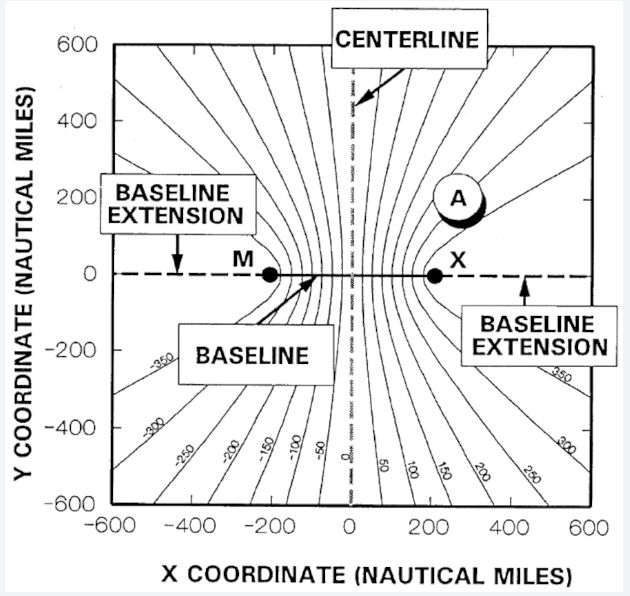
Mathematically, these curves are hyperbolas. On a sphere (rather than the plane used in Figures 3 and 4) these would be spherical hyperbolas, while on the slightly nonspherical earth these would be spheroidal hyperbolas. Readers accustomed to looking at relatively large-scale loran overprinted nautical charts may be surprised at the curvature of the LOPs shown in Figure 4. Over the short distances covered by a large-scale charts the curvature of the loran LOPs is much less apparent.
The locus of points that have a constant difference in distance from a master and secondary station describes a mathematical curve termed a hyperbola.
To illustrate, suppose that point A were located at the point shown in Figure 4, A = (271,9, 200). From equation (3), the distance from point A to the secondary would be approximately 212,5 nautical miles. And, from equation (2), the distance from point A to the master would be approximately 512,5 nautical miles. Point A, therefore, is 300 miles closer to the Xray secondary than to the master. Figure 4 also shows the locus of all such points 300 miles closer to the secondary than to the master – this contour is a hyperbola labeled with the number 300. Thus, if we could determine that we were 300 miles closer to the secondary than to the master, we would be located somewhere along this hyperbolic LOP (300).
These hyperbolic LOPS are all curved, with the exception of the LOP where the difference in distance is exactly zero. This is termed the centerline of the system, and is a “straight” line (rather than a curve) that bisects the baseline. On the curved surface of the earth the centerline is actually a great circle oriented at right angles to the baseline. The baseline extension is also shown in Figure 4.
Equivalence Between Distance and Time
The contours in Figure 4 are labeled in terms of distance, but (assuming a constant speed of signal propagation) could equally well , be labeled in terms of time difference (TD). All that is necessary to calculate the theoretical time difference for any point in Figure 4 is the speed of signal propagation and the CD of the Xray secondary. To a first approximation This assumption is refined below as various corrections are introduced.x, loran signals travel at the speed of light – it takes approximately 6,18 usec for the signal to travel one nautical mile.
Now consider point A again in Figure 4. The distance from the master to point A is 512,5 NM, so the signal from the master would take approximately 6,18 (512,5) = 3 167 usec to reach a vessel at point A. The arrival of this signal starts the TD measurement in the vessel’s loran receiver. When will the signal from the secondary arrive? Recall that the secondary transmits after an emission delay, equal to the baseline travel time plus the secondary coding delay. The master and Xray secondary are 400 miles apart in this illustration, so the baseline travel time (or baseline length in usec) is approximately 6,18 (400) = 2 472 usec. Assuming a CD for this secondary of 11 000 usec Recall that EDs and CDs for each secondary in each chain are given in “Data Sheets and Coverage Diagrams”.x, the Xray secondary would transmit 2 472 + 11 000 = 13 472 usec after the master. This signal must travel approximately 212,5 NM to reach the vessel at point A, a travel time of 6,18 (212,5) = 1 313 usec. Thus, in this example, the signal from Xray would arrive 13 472+1 313 = 14 785 usec after the master transmission. The observed TD at the vessel is this time, 14 785 usec, minus the time that the master signal arrives at the vessel, previously calculated as 3 167 usec. The theoretical TD (based upon these assumptions) at the vessel is 14 785-3 167 = 11 618 usec. This calculation is summarized in Table 2 and the time lines are shown diagrammatically in Figure 5.
| Table 2. Theoretical calculation of time delay at point “A” | |
|---|---|
| Propogation | Time (usec) |
| Master to Secondary (400 NM) – baseline travel time | 2 472 |
| Secondary Coding Delay (CD) | 11 000 |
| Secondary to Vessel (212,5 NM) | 1 313 |
| Master to Vessel (512,5 NM) | -3 167 |
| Measured Time Difference at Vessel | 11 618 |
| Alternative calculation | |
| Baseline Travel Time | 2 472 |
| Secondary Coding Delay | 11 000 |
| Difference in Distance (300) Between Master and Secondary Stations and Vessel | -1 854 |
| Measured Time Difference at Vessel | 11 618 |
| NOTE: Calculations shown here are only approximate, SFs and ASFs, for example, are not included here. | |
Other sources of system error remain, but these corrections are usually sufficient to ensure 0,25 NM absolute accuracy.
Loran LOPs can be displayed as distance differences or equivalently as TDs. Because TDs are measured on the receiver, these are shown on loran overprinted charts.
Returning now to Figure 4, the LOP on which point A is located could be labeled as 300 NM or equivalently as 11 618 usec. Any point on this LOP is 300 miles closer to the Xray secondary. Likewise (given the assumed CD), at any point on this same line, the theoretical TD would also be 11 618 usec. Because it is the TD rather than the difference in distance that is measured, it is much more convenient to label the loran overprinted nautical chart with the TD. More typically the LOPs shown on a loran overprinted chart would be evenly spaced every 5 or 10 usec (See Loran-C Charts and Related Information“Loran-C Charts Key Components and Navigation Techniques”).
With a few added complexities (discussed below) to account for a nonconstant speed of signal propagation, this is the exact procedure used for calculation of the theoretical location of the TDs on the nautical chart.
Though tedious, calculation of the location of lines of constant time difference is a straightforward exercise in geometry. To a first approximation, lines of constant difference in distance from two stations are also lines of constant TD.
More Exact Calculations
The foregoing calculations assume a constant speed of propagation of the Loran-C signal. This simplifying approximation is very nearly correct, but would result in position inaccuracies that exceed the designed accuracy limits of the Loran-C system. Therefore, it is necessary to refine this approximation.
Conventionally, this refinement process amounts to applying various corrections to either the speed of propagation of the loran signal or equivalently the predicted time required for the signal to traverse a specified distance. Typically three correction factors, termed phase factors, are applied. These are defined and summarized in Table 3.
| Table 3. Phase factor corrections necessary to ensure Loran-C accuracy specifications are met | |||
|---|---|---|---|
| Quantity | Primary Phase Factor | Secondary Phase Factor | Additional Secondary Phase Factor |
| Abbreviation | PF | SF | ASF |
| Brief Description | A correction to a Loran-C reading due to signal propagation through the atmosphere as opposed to propagation through free space. | The amount, in usec, by which the predicted time difference of a pair of Loran-C signals that travel over all-seawater paths differs from that of signals that travel through the atmosphere. | The amount, in usec, by which the time difference of an actual pair of Loran-C signals that travel over terrain of various conductivities differs from that of signals which have been predicted on the basis of travel over all-seawater paths. |
| Function of | Atmospheric Index of Refraction | Conductivity and permittivity of seawater – time delay a function of distance. | Specific paths between master, secondary, and vessel. |
| Included on Loran-overprinted Charts | Yes | Yes, on most modern receivers, check owner’s manual for individual set. | |
| Included in Lat/Long Conversions on Loran-C Receivers | Yes | Yes, on most modern receivers, check owner’s manual for individual set. | |
| Additional Information Available From | See Glossary for details | See DMAHTC Loran-C Correction Tables, for various chains and secondaries. | |
Primary Phase Factor (PF)
The first of these factors is termed the primary phase factor (PF), and accounts for the fact that the speed of propagation of the signal in the atmosphere is slightly slower than in free space (vacuum). According to Bowditch, the speed of light in vacuum is 161 875 NM/sec (equivalent to 6,17761 usec/NM), whereas in the atmosphere the speed is slowed slightly to 161 829 NM/sec (equivalent to 6,17936 usec/NM). This speed difference is related to the fact that the atmosphericindex of refraction is slightly greater than unity. All Loran-C overprinted charts and loran receivers incorporate the PF correction.
Secondary Phase Factor
The second correction factor, termed the secondary phase factor (SF), reflects the fact that the loran groundwave is further retarded when traveling over seawater as opposed to through the atmosphere. When the Loran-C signals are transmitted, part of the electromagnetic wave is in the air, and part penetrates the earth’s surface. Seawater is not as good a electrical conductor as air, so the signals are slowed as they travel over seawater. The amount of time required for travel over a specified distance will exceed that calculated using the PF by an amount equal to the SF. SF is applied as acorrection term to the required travel time rather than as an adjustment to the propagation speed of the signals. Several equations for SF have been proposed, such as the so-called Harris polynomials shown below which relate the SF to the distance traveled, d (in statute miles):
Table 4 shows the PFs and SFs (from equation 7) applied to the approximate calculation given in Table 4. For this example, the more exact calculation differs little from the approximate calculation, but (depending on the position within the coverage area) these differences could be numerically larger. As with PFs, SFs are incorporated into all Loran-C overprinted charts and commercial receivers.
Additional Secondary Phase Factor (ASF)
Application of the PF and SF enables calculation or loran TDs over an all-seawater path. In practice (see, e. g., Figure 2), loran signals travel over a mixed path; partially over land of various conductivities, and partially over seawater. The correction arising from the additional retardation of the signal is termed the additional secondary factor (ASF). ASF is the least predictable of the phase factors. Many things affect the value of ASF along a signal transmission path, including conductivity of the soil (which itselfvaries with the temperature and water content of the soil), distance traveled over land, etc. The accuracy of a conversion from Loran-C TDs to latitude/longitude (discussed in Loran-C Position Determination and Accuracy“LORAN-C System: Accuracy and Position Determination” and Loran-C Charts and Related Information“Loran-C Charts Key Components and Navigation Techniques”) depends critically on the value of ASF used in the mathematical signal propagation model.
ASF is generally calculated by considering the overall path as separate segments, each having a uniform conductivity value. The ASF of each segment can be computed and then the composite ASF is derived. A popular method of doing this is called Millington’s method, reviewed in Exploring Loran-C Millington’s Method“Loran-C Millington’s Method – Conductivity and Propagation”. Another method of determining ASF is to measure the TDs at a point, compute the TDs at the same point using a mathematical model which assumes an all seawater propagation path, and then determine the difference between the measured and computed TDs. A finite number of such measurements can be made and extrapolated to cover the areas between measurements. ASFs “measured” in this fashion tend to be more accurate than those computed by Millington’s method. ASFs at a fixed point in the coverage area actually vary with time. To achieve optimum accuracy these – temporal ASF changes must be taken into account. ASF variations with time are chiefly caused by changes in soil conductivity due to seasonal weather variations, daylnight temperature variations, and local weather activity (thunderstorms, droughts, etc.).
| Table 4. Theoretical calculation of time delay at point “A” using PFs and SFs | |||
|---|---|---|---|
| Propogation | PF (usec) | SF (usec) | Time (usec) |
| Master to Secondary (400 NM) – baseline travel time | 2 471,74 | 1,25 | 2 472,99 |
| Secondary Coding Delay | NA | 11 000,00 | |
| Secondary to Vessel (212,5 NM) | 1 313,11 | 0,55 | 1 313,67 |
| Master to Vessel (512,5 NM) | 3 166,92 | 1,68 | -3 168,61 |
| Measured Time Difference at Vessel | 11 618,05 | ||
In summary, speed and phase of Loran-C signals are affected by several physical parameters. The primary, secondary, and additional secondary phase factors (PF, SF, and ASF) account for changes due to air, seawater, and land paths, respectively.
ASF Tables
As can be seen from Exploring Loran-C Millington’s Method“Loran-C Millington’s Method – Conductivity and Propagation”, computation of even average (let alone time varying) ASFs is quite tedious, and requires a substantial data base describing the relevant conductivity of land or mixed landwater paths. Fortunately these ASFs are incorporated into most Loran-C overprinted charts and also many Loran-C receivers.
Although ASF corrections are incorporated into most (but not all) modern Loran-C receivers, the user should remember that the government is responsible for the accuracy of the ASFs incorporated into ASF tables (see below) and loran overprinted charts. The government is not responsible and cannot guarantee the quality of the ASF data bases used in Loran-C receivers, these are strictly the responsibility of the manufacturer.
Additionally, ASFs can be found in a set of tables, called Loran-C Correction Tables, prepared and published by the Defense Mapping Agency, Hydrographic/Topographic Center (DMAHTC). These tables are published in a series of volumes, one for each loran chain. Each volume is organized into a set of pages for each station pair (master and secondary) or rate within the chain. Further, each page of corrections in the table covers an area three degrees in latitude by one degree of longitude. An index permits rapid determination of the appropriate page in the table to find ASFs of interest.
Table 5 provides an excerpt of a Loran-C Correction Table for the NEUS (9960) chain and master-Whiskey station pair. This page covers an area off the mouth of the Delaware Bay between latitudes of 36° 0′ N and 39° 0′ N, and longitudes 74° 0′ W and 75° 0′ W. Large land bodies and areas outside the CCZ are represented by blank spaces on the pages (see Table 5).
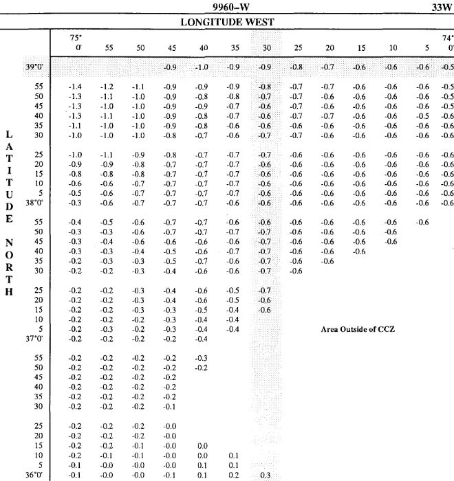
ASF corrections given in this table are to be applied to the measuredTDs, andcan be positive or negative. Negative values are prefixed with a minus (-) sign, while positive values are shown without sign. In some cases, a negative sign precedes a zero value; this results fromrounding off a value slightly less than zero and indicates the trend of the correction.
Use of Tables
According to DMAHTC, “ASF tables are published primarily for precision navigators who utilize electronic computers to convert Loran-C time differences to geographic coordinates.” These tables can also be used by navigators using manual plotting methods for Loran-C navigation.
ASF corrections are typically small (no more than ±4 usec), but can be significant for precise navigation, a point illustrated below.
The ASF correction table can be entered by using the vessel’s dead reckoning (DR) position, indicated loran position, or position determined by other means. ASFs are added algebraically to the measured (observed) TD of the station pair. For example, suppose that the vessel were located at the approximate position 39° 0′ N and 74° 30′ W, and that the ASF for the Whiskey station pair were desired. From Table 5 it can be seen that the ASF is -0,9 usec. Thus, in this instance 0,9 usec should be subtracted from the observed TD to obtain a corrected TD.
ASF corrections should be used with caution for areas within ten nautical miles of land (coastline effect) and should not be used with charts that provide a corrected lattice.
Care should be taken to ensure that the correct table (hence chain) is used, and that the correction station pair is considered. Table 6, for example, shows how the ASF correction (for the same latitude and longitude used in the above illustration) varies with the secondary station and chain. Assuming the location given, the correction appropriate for the Xray secondary in the 9960 chain would be 2,9 usec, compared to only 0,3 usec if the 8970 chain were used. It is particularly important to use the right table (correct chain and station pair) when determining ASF corrections.
| Table 6. ASFs depend upon the observer’s location, chain, and secondaries used | ||||
|---|---|---|---|---|
| Approximate Position: L: 39° 00′ N, Lo: 74° 30′ W | ||||
| Chain | Secondary | |||
| X | W | Y | Z | |
| 9960 | 2,9 | -0,9 | 1,9 | -0,3 |
| 8970 | 0,3 | 0,0 | Not given | N/A |
Lest the reader conclude that all this emphasis on refined calculations is much ado about nothing, the accuracy of the predicted LOP is a key determinant of the accuracy of the loran position. Loran-C accuracy and its determinants are explored in some detail in Loran-C Position Determination and Accuracy“LORAN-C System: Accuracy and Position Determination”. One important determinant of accuracy is the gradient of the LOP. Technically, the gradient is the number of ft (meters, yds, etc.) position difference divided by the number of microseconds. As shown in Loran-C Position Determination and Accuracy“LORAN-C System: Accuracy and Position Determination”, these gradients are smallest on the Loran-C baseline, andincrease throughout the coverage area. Even for positions located on the baseline, however, the gradient is nearly 492 ft/usec. So an ASF correction of 3 usec, for example, corresponds to aposition difference of at least 1 476 ft in position – and perhaps several times greater. Concern over appropriate ASF corrections is not merely a technicalquibble.
ASF tables are typically not interpolated, as the ASF functions are generally not linear. Figure 6, for example, shows smoothed contours of equal ASF for the data displayed in Table 5.
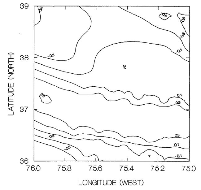
As can be seen, there are numerous ridges, saddle points, and local maxima and minima in the surface described by the data. Simple linear interpolation would not offer any meaningful increase in accuracy for such a complex surface. Rather, the correction nearest to the vessel’s approximate latitude and longitude should be applied to the appropriate time difference.
ASF corrections may change over time, as new and more accurate corrections are determined, so the latest volume should be consulted. According to some observers (Melton, 1986) the average ASFs are changing in such areas as Florida’s west coast, due to the construction of high-rise buildings there.
ASFs (and loran accuracy in general) are much less certain in the vicinity of the coastline (coastline effect). DMAHTC recommends that ASF corrections be used with caution for areas within 10 NM of a coastline.
Groundwave versus Skywave Propagation
Radio energy from a Loran-C transmitter emanates in all directions. The pulsed Loran-C signal, therefore, may reach the observer by many propagation paths. These paths are conveniently grouped into two major categories:
- groundwave,
- and skywave.
The groundwave signal propagates in the atmospheric medium below the ionosphere (an electrified layer of the atmosphere) and is relatively well understood and quite predictable.
However, the signal strength of the groundwave is attenuated as it follows the contour of the earth. At great distances from the transmitter, the groundwave signal is substantially attenuated.
Skywaves consist of that component of the Loran-C signal which travels to the observer via reflection from the ionosphere which is actually comprised of several reflecting layers, assigned letter symbols in conventional nomenclature. For the 100 kHz frequency of the Loran-C, this reflection will take place in the lower E or D region of the ionosphere. The reflection height will vary from approximately 60 kilometers during daylight, to approximately 90 kilometers at night. From the geometry of the reflection, it is obvious that the skywave signal must travel a longer distance to reach an observer and will arrive after the corresponding groundwave – generally after a time lapse of from 35 usec to 1 000 usec after the groundwave (depending upon the height of the reflecting layer in the ionosphere). Because skywaves do not travel over the surface of the earth, these are not attenuated to the same extent as the groundwave. In consequence, at long distances, the skywave signal may be very much stronger than the groundwave signal. The skywave can cause distortion of the received groundwave signal in the form of fading and pulse shape changes – generally given the name “skywave cantamination.”
Although it is possible to develop position information from skywave signals (and, indeed, skywaves were used in early loran), the most accurate navigation requires the use of the loran groundwave. (Use of skywaves for navigation is discussed briefly in Use of Skywaves for Navigation“Harnessing Skywaves for Navigation With Loran-C”.)
The reason why groundwaves are preferred over skywaves for accurate navigation is that the propagation conditions (in the ionosphere) are not stable, but change from day-to-day and even hour-to-hour, whichvastly complicates the problem of prediction of arrival times for skywaves. The skywave, therefore, is generally regarded as a “nuisance,” and the Loran-C system has been designed in part to minimize the possible influence of skywaves on groundwave reception and tracking.
Pulse Architecture and Related Technical Matters
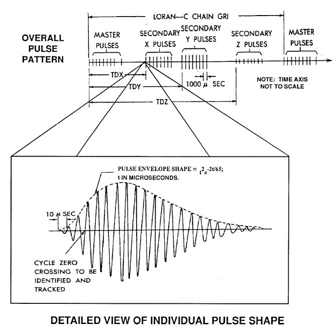
It is noted above that the Loran-C system uses pulsed transmission-nine pulses for the master and eight pulses for the secondary transmissions. Figure 7 shows this overall pulse pattern for the master and three secondary transmitters (Xray, Yankee, and Zulu). Shown also in Figure 7 is an “exploded” view of the Loran-C pulse shape.
pulse shape for Loran-C transmission
It consists of sine waves within an envelope that might loosely be described as “teardrop shaped,” and is referred to technically as a t-squared pulse. (The equation for the envelope is also included in Figure 7.) This pulse will rise from zero amplitude to maximum amplitude within the first 65 usec and then slowly trails off or decays over a 200-300 usec interval. The pulse shape is designed so that 99 % of the radiated power is contained within the allocated frequency band for Loran-C of 90 kHz to 110 kHz.
The rapid rise of the pulse allows a receiver to identify one particular cycle of the 100 kHz carrier. Cycles are spaced approximately 10 usec apart. The third cycle of this carrier within the envelope is used when the receiver matches the cycles. The third zero crossing (termed the positive 3rd zero crossing) occurs at 30 usec into the pulse. This time is both late enough in the pulse to ensure an appreciable signal strength and early enough in the pulse to avoid skywave contamination from those skywaves arriving close after the corresponding groundwave.
| Table 7. Technical and other reasons for several key Loran attributes | |
|---|---|
| Feature | Reason for Inclusion |
| Pulsed Transmission | To save on prime power required for transmission and to facilitate signal identification and precise timing. Multiple pulses were selected over single pulses to increase the average power. |
| Different Number of Pulses on Master versus Secondary | Facilitate identification of master. On modern commercial receivers phase coding is now used for this purpose. |
| Phase Coding | Reduce the effects of skywaves on the loran groundwave. Also assists in identifying master from among secondaries. |
| Pulse Shape | Selected so that 99 % of the radiated power is contained within the allocated frequency band of 90-110 kHz. Fine structure in pulse shape enables cycle matching to be used, increasing accuracy of timing relative to envelope matching. |
| Standard Zero Crossing | Compromise made; selected to be early enough in the pulse to lessen effects of skywave contamination. Selected as 30 usec in normal use (without cycle step). |
| Blink Codes | To provide users with indications of loran system accuracy and reliability. Secondary blink is detectable by the majority of users to indicate low power, improper TDs, ECD out of tolerance, and/or improper phase code or GRI. |
| 90-110 kHz Frequency | Avoid interference with other users of the frequency spectrum and ensure adequate (relatively long) range. The spacing between each cycle of 100 kHz is approximately 10 usec, and technologically it was easier to design equipment to measure time in tenths of a microsecond. |
| Relative Time Measurements | Simplify and reduce costs of receivers (no absolute time reference required). Eliminate the need to account for all variances in propagation time (e. g., those arising from use of notch filters) in order to have accurate system. |
| Overall, a complex system at a detailed level. But these complexities are essential to create highly accurate, reliable, long-range system that is easy to use. | |
Phase Coding
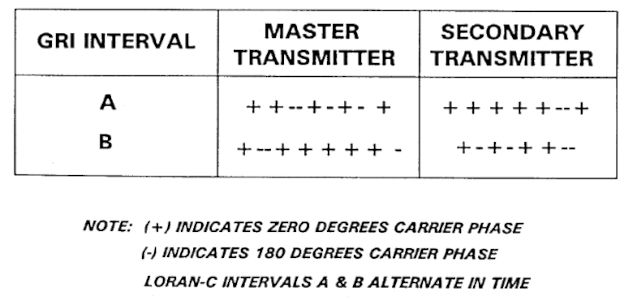
Within each pulse group from the master and secondary stations, the phase of the radio frequency (RF) carrier is changed systematically from pulse-to-pulse in the pattern shown in Figure 8. This procedure is known as phase coding. The patterns “A” and “B” alternate in sequence. The pattern of phase coding differs for the master and secondary transmitters. Thus, the exact sequence of pulses is actually matched every two GRIs – an interval known as a phase code interval (PCI) Technically speaking, the exact sequence of loran pulses does not repeat every GRI, but rather every PCI.x.
Phase coding enables the identification of the pulses in one GRI from those in an earlier or subsequent GRI. Just as selection of the pulse shape and standard zero crossing enable rejection of certain skywaves, phase coding enables rejection of others; late airway skywaves will have adifferent phase code from the groundwave. Because the master and secondary signals have different phasecodes, these can be distinguished by the loran receiver. Phase coding also offers other technical benefits.
Blink Coding
The Loran-C system also permits the secondary transmissions (more specifically the first two pulses of the secondary pulse group) to “blink.” This secondary blink can be detected by the loran receiver, and is used to warn users that the loran signal is unreliable and should not be used for navigation. (The specifics of the blink display differ from receiver-to-receiver-in some cases a blink alarm on the receiver will light, in others the displayed TDs simply blink on and off.) Blink alarms warn that the signal power, TD, or ECD is out-of-tolerance (OOT) and/or that an improper phase code or GRI is being transmitted. The blink coding contributes significantly to the integrity of the loran system.
When secondary blink is enabled, the first two pulses of the affected secondary are blinked at a four-second cycle; about 3,6 seconds off and about 0,4 seconds on. Secondary blink is used to advise users of potential problems. The loran system also has the capability to blink the master signal. Master blink is used for internal communications, and does not indicate a system malfunction. Most modern user receivers are not programmed to detect master blink.
Concluding Comments
Table 7 summarizes some of the key technical features of the Loran-C system and reasons for their inclusion. At a detailed level, this system is highly complex, but these complexities are essential tocreate a highly accurate, reliable, and easy to use long-range system.

- Abramowitz, M., et al. “Approximate Method for RapidLoran Computation,” Navigation; Journal of the Institute of Navigation, Vol. 4, No. 1, March 1954, pp. 24-27.
- Alexander, G. “The Premier Racing Tool,” Ocean Navigator, Issue No. 20, Jul/Aug 1988, pp. 37, er seq.
- Anonymous. “Loran: Installation Pitfalls, and How Friendly Should Your Loran Be?” Practical Sailor, Vol. 11, No. 24, December 15, 1985, pp. 1, et seq.
- Anonymous. Manual on Radio Aids to Navigation, International Associationof Lighthouse Authorities, Nouvelle Adresse, 13 Rue Yvon-Villarceau 75 116, Paris, 1979.
- Appleyard, S. F. Marine Electronic Navigation. Routledge and Kegan Paul Ltd., Boston, MA, 02108, 1980.
- Ashwell, G. E., B. G. Pressey, and C. S. Fowler. The Measurement of the Phase Velocity of Ground Wave Propagation at low Frequencies Over a Land Path. Proceedings of the Institute of Electrical Engineering (London) 100 Part III, 1953.
- Bedford Institute of Oceanography. Loran-C Receiver Performance Tests, Bedford Institute of Oceanography, P. O. Box 1006, Dartmouth, NovaScotia, Canada, B2Y 4A2.
- Blizard, M. M. et al. Harbor Monitor System Final Report, CG-D-17-87, ADA 183 477, Dec. 1986, Available through the National Technical Information Service, Springfield, VA, 22161.
- Blizard, M. M., Lt. and CWO 3 D. C. Slagle. Differential Loran-C System Final litter, Draft, United States Coast Guard, January 1987.
- Blizard, M. M. and D. C. Slagle, “Loran-C West Coast Stability Study,” Proceedings of the Fourteenth Wild Goose Technical Symposium, Wild Goose Association, Bedford, MA, 1985.
- Brogdon, B., “Loran Expansion,” Ocean Navigator, Issue No. 42, SeptfOct 1991, pp. 87, et seq.
- Brogdon, W. “Loran Hook, a Little Known, Foible Explained,” Boating, August 1991, p.42.
- Brogdon, W. “Electronic Errors,” Ocean Navigator, Issue No. 40, June 1991,pp. 70, etseq.
- Brogdon, W. “Pathfinders,” American Hunter, Vol. 19, No. 7, July 1991.
- Burt, W. A., et al. Mathematical Considerations Pertaining to the Accuracy of Position, Location, and Navigation Systems, Part I, Stanford Research Institute, 1966. Available from National Technical Information Service, AD-629609, US Department of Commerce, 5825 Port Royal Road, Springfield, VA 2215 1.
- Canadian Coast Guard, Aids and Waterways Branch. A Primer on Loran-C, Ottowa, Ontario, Canada, 1981.
- Connes, K. The Loran, GPS & NAVICOMM Guide, Butterfield Press, 1990.
- Culver, C. “A New High Performance Loran Receiver,” Proceedings of the Sixteenth Annual Technical Symposium, The Wild Goose Association, 20-27 October 1987, pp. 282, et seq.
- Dahl, B. “Adopting Loran-C to Everyday Navigation,” Cruising World,May 1983,pp. 40-45.