Uncover the latest advancements in DVB-S2 modulation and its extensions in this comprehensive review. Explore key concepts such as modulation and FEC principles, Eb/No metrics, and the role of filters and roll-off factors. Learn about the implications of H.265 coding, innovative ground-side technologies like Carrier ID and Intelligent Inverse Multiplexing, and how these enhancements are shaping the future of satellite communications.
We noted in Exploring the Future of Satellites“Trends, Technologies and Applications of Modern Satellites” that business factors that impact the industry at press time include the user’s (and operator’s) desire for higher overall satellite channel and system throughput. Evolving applications, whether in the context of the delivery of High Definition (HD), Ultra HD, or Internet access for people on the move (on airplanes or ships), drive the operator’s need for higher channel throughput. Beyond the intrinsic radio channel behavior, modulation and error correction dictate, in large measure, the performance of the satellite link, the effective channel throughput, and the service availability that one is able to obtain over the satellite link.
Enhanced modulation schemes allow users to increase channel throughput: refined modulation and coding (MODCOD MODCOD is also written as modcod.x) techniques are now being introduced as standardized solutions embedded in next-generation modems that provide more bits per second per unit of spectrum. Specifically, extensions to the well-established baseline DVB-S2 standard are now being introduced in the market. Adaptive coding that is incorporated with the new modulation schemes enables more efficient use of the higher frequency bands (e. g., Ka) that are intrinsically susceptible to rain-fade. Other ways of achieving higher application-level throughput are discussed in the next article.
The first part of the article provides a foundation for the modulation and Forward Error Correction (FEC) discussion; the second part then focuses on the recent advances for ground-based elements of the satellite ecosystem, specifically DVB-S2 extensions known as DVB-S2X. The last part of the chapter briefly covers Carrier ID. The concept of Intelligent Inverse Multiplexing for satellite applications is also discussed. Brief mention is made of High Efficiency Video Coding (HEVC)/ITU-T H.265, as another aspect of ground-related advances expected to impact the industry (a topic discussed in greater details in M2M Developments and Satellite Applications“Exploring Innovations and Applications of M2M Technology”).
A Review of Modulation and FEC Principles
We review some fundamental technical principles in this introductory section, before looking at the latest advancements in this arena.
Eb/No Concepts
Eb is a measure of the bit energy; Eb = Pavg/Rb, where Rb is the bit rate. Eb/No, the ratio of bit energy to noise power spectral density measured in decibel, is a commonly used parameter to compare digital systems, namely, modulation outcomes.
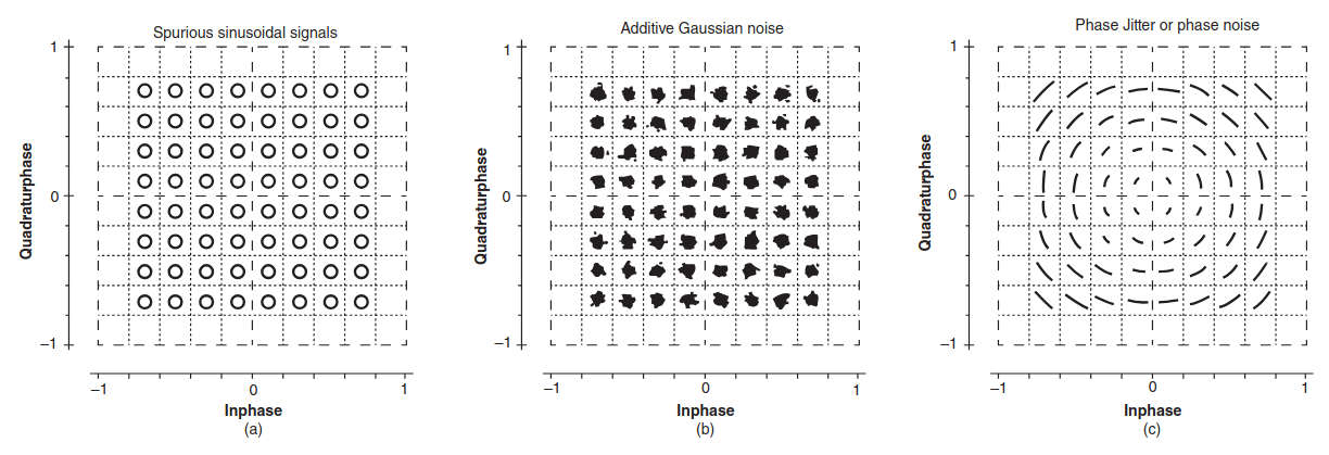
Key impairments that impact demodulation are the following (refer to the Glossary for the definition of these terms):
- Additive Gaussian noise;
- Amplitude imbalance;
- Carrier suppression or leakage;
- Interferers;
- Phase error;
- Phase jitter and/or phase noise.
If the input signal is distorted or greatly attenuated (e. g., see Figure 1), the receiver can no longer recover the symbol clock, demodulate the signal, and/or recover the information. In some cases, a symbol will fall far away from its intended constellation position that it will cross over to an adjacent position; the in-phase (I) and quadrature (Q) level detectors used in the demodulator would misinterpret such a symbol as being in the wrong location, resulting in bit errors. In this context, note that Quadrature Phase Shift Keying (QPSK) is not as spectrally efficient as, say, 8-PSK or 16-QAM (Quadrature Amplitude Modulation), but the modulation states are much farther apart and the system can thus tolerate a lot more noise before suffering symbol errors.
To improve the Bit Error Rate (BER) performance beyond what the basic Eb/No provides (or to optimize operation at a given fixed Eb/No), one needs to employ various FEC techniques. FEC is a system of error control for data transmission wherein the receiving device has the capability to detect and correct, in a simplex mode (1-way communication channel), any character or code block that contains fewer than a predetermined number of symbols in error.
FEC is accomplished by adding bits to each transmitted character or code block, using a predetermined algorithm (FEC is described in more detail in the next section). Figure 2 depicts the general behavior of a modulation scheme used without and with FEC; note that if there is a higher number of redundant bits, a given BER can be achieved with a lower Eb/No (lower Eb or higher No).
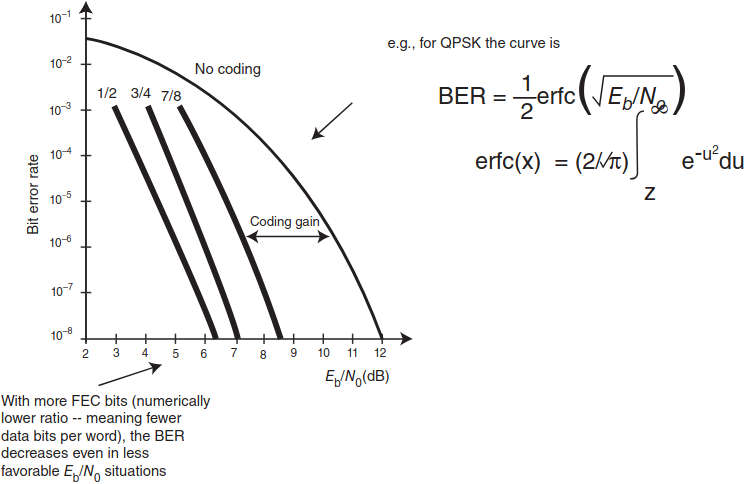
Also, note that the performance gradients become such that even the least improvement in Eb/No can have a major impact on BER for a given FEC technique.
Some useful observations related to Eb/No are as follows.
- Bit rate = (symbol rate) × (number of bits sent per symbol). For example, if two bits are transmitted per symbol (e. g., in QPSK), the symbol rate is half of the bit rate.
- No is the noise density, namely, the total noise power in the frequency band of the signal divided by the bandwidth (BW) of the signal; No = Pn/Bn with Pn = Noise Power (the units here in Joules) and Bn = Noise BW. No is measured in W/Hz. It is the noise power in 1 Hz of BW.
- 0 dB means the signal and noise power levels are equal and a 3 dB increment doubles the signal relative to the noise. Hence, if the power increases, Eb/No increases; if the noise increases, Eb/No decreases.
- A related concept is Eb/No (also measured in dB). It represents the ratio of signal energy per symbol to noise power spectral density.
where:
- SNR – Signal-to-Noise Ratio;
- Es – Signal energy (Joules);
- Eb – Bit energy (Joules);
- No – Noise power spectral density (Watts/Hz);
- Tsym – Symbol period parameter of the block in Es/No mode;
- k′ Number of information bits per input symbol (which is not to be confused with Boltzmann’s constant k);
- Tsamp – Inherited sample time of the block, in seconds.
Note that signal-to-noise ratio (SNR) is a measure of the quality of an electrical signal, usually at the receiver output. It is the ratio of the signal level to the noise level, measured within a specified BW (typically the BW of the signal). The higher the ratio, the better the quality of the signal. It is expressed in dB.
The relationship between Es/No and SNR can be derived as follows:
where:
- Tsym – Signal’s symbol period;
- Tsamp – Signal’s sampling period;
- S – Input signal power, in Watts;
- N Noise power, in Watts;
- Bn – Noise BW, in Hertz;
- Fs – Sampling frequency, in Hertz.
Note that Bn = Fs = 1/Tsamp.
One can show that:
where erfc, that is, the complimentary error function, describes the cumulative probability curve of a Gaussian distribution, namely:
Note that in an analog environment, the measures of interest are C/N (carrier power to noise power ratio) and C/No. These two measures are employed the same way Eb/No is used in digital environments. C/N is the carrier power in the entire usable BW, C/No is carrier power per unit BW.
One can convert Eb/No to C/N using the equation:
where:
- B – Channel BW;
- Rb – Bit rate.
When all the terms are in decibel, then one has:
FEC Basics
Along with modulation, FEC drives, in large measure, the performance of the satellite link, the effective channel throughput, and the service availability that one is able to obtain. FEC is required to achieve high performance in satellite links given the typical presence of high levels of noise and interference. FEC mechanisms can detect and correct a (certain) number of errors without retransmitting the data stream; this is done utilizing coded extra bits added to the transmitted data blocks.
Figure 3 depicts a basic diagram of FEC encoding.
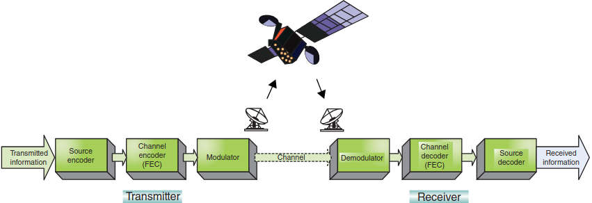
A FEC encoder adds redundancy to the data message at the transmitter according to certain defined rules. The FEC decoder at the receiver uses the knowledge of these rules to identify and, if possible, correct any errors that have accrued during transmission. FEC codes take a group of g data packets and generate h = n−g parity packets. The total block size n consists of the g data and h parity packets. Once the parity packets have been computed, the block is then transmitted. The block format may vary according to the application.
Typically, one has to be concerned with the following parameters:
- g – Number of data packets per block;
- h – Number of parity packets per block where h = n−k′′;
- n – Number of total packets per block;
- R – % of total BW used for redundancy;
- TFEC – FEC latency.
There are two basic types of FEC codes (also see Table 1):
- Block codes. In these algorithms the encoder processes a block of message symbols and then outputs a block of codeword symbols. Broadly deployed Bose–Chaudhuri–Hocquenghem (BCH) codes belong to the family of block codes, as do the Reed–Solomon (RS) codes. The input to a FEC encoder is some number k of equal-length source symbols. The FEC encoder generates n−k redundant symbols yielding an encoding block of n encoding symbols in total (composed of the k source symbols and the n−k redundant symbols). Namely, a (n, k) linear block encoder takes k-bit block of message data and appends n−k redundant bits algebraically related to the k message bits, producing an n-bit code block. The chosen length of the symbols can vary on each application of the FEC encoder, or it can be fixed. These encoding symbols are placed into packets for transmission. The number of encoding symbols placed into each packet can vary on a per packet basis, or a fixed number of symbols (often one) can be placed into each packet. Also, in each packet is placed enough information to identify the particular encoding symbols carried in that packet. A block FEC decoder has the property that any k of the n encoding symbols in the encoding block, which is sufficient to reconstruct the original k source symbols. On receipt of packets containing encoding symbols, the receiver feeds these encoding symbols into the corresponding FEC decoder to recreate an exact copy of the k source symbols. Ideally, the FEC decoder can recreate an exact copy from any k of the encoding symbols.
- Convolution codes. In these algorithms, instead of processing message symbols in discrete blocks, the encoder works on a continuous stream of message symbols and simultaneously generates a continuous encoded output stream. Convolutional coding is a bit-level encoding technique rather than block-level techniques such as RS coding. These codes get their name because the encoding process can be viewed as the convolution of the message symbols and the impulse response of the encoder.
The performance improvement that occurs when using error control coding is often measured in terms of coding gain. Let us suppose an uncoded communications system achieves a given BER at an SNR of 35 dB.
| Table 1. Key FEC Families | |
|---|---|
| FEC Algorithm | Definition/Characteristics |
| Bose-Chaudhuri-Hocquenghem (BCH) | A block code developed by the three named researchers (BCH codes were invented in 1959 by Hocquenghem, and independently in 1960 by Bose and Ray-Chaudhuri.). It is a generalization of the Hamming codes. BCH encodes k data bits into n code bits by adding n−k parity checking bits. Galois Fields (GF) concepts are used. BCH codes are cyclic codes over GF(q) (the channel alphabet) that are defined by a (d−1) × n check matrix over GF(qm) (the decoder alphabet): where: • is an element of GF(qm) of order n; Rows of H are the first n powers of consecutive powers of . |
| Reed–Solomon (RS) | Reed–Solomon codes are BCH codes where decoder alphabet = channel alphabet. The Reed–Solomon codec (coder–decoder) is a block-oriented coding system that is applied on top of the standard Viterbi coding. It corrects the data errors not detected by the other coding systems, significantly reducing the bit error rates (BERs) at nominal signal-to-noise levels (4–8 dB Eb/No). Bandwidth expansion is small, following the increase in code rate in the range 6–12 %. Typically, Reed–Solomon coding is used in areas where sensitivity to transmission errors is particularly high. The “Reed–Solomon + Viterbi” option is particularly well suited to data communication applications with little or no packet acknowledgment or no packet retransmission, such as is the case in satellite communication. |
| Viterbi Algorithm | The term Viterbi specifically implies the use of the Viterbi Algorithm (VA) for decoding, although the term is often used to describe the entire error correction process. The encoding method is referred to as convolutional coding or trellis-coded modulation. A state diagram illustrating the sequence of possible codes creates a constrained structure called a trellis. The coded data is usually modulated; hence, the name trellis-coded modulation. The outputs are generated by convolving a signal with itself, which adds a level of dependence on past values. |
| Turbo Codes | In 1993, a new coding and decoding scheme, dubbed “Turbo codes” by its discoverers, was introduced that achieves near-capacity performance on additive white Gaussian noise channel. This technique was based in the use of two concatenated convolutional codes in parallel. After the introduction of Turbo codes the industry has seen the emergence of a plethora of codes that exploit a Turbo-like structure. The common aspect of all Turbo-like codes (TLC) is the concatenation of two or more simple codes separated by an interleaver, combined with an iterative decoding strategy. Members of the TLC family are: • Parallel Concatenated Convolutional Codes (PCCC) (this is the classical Turbo code); • Serially Concatenated Convolutional Codes (SCCC); • Low-Density Parity Check Codes (LDPC), and; • Turbo Product Codes (TPC). |
Imagine that an error control coding scheme with a coding gain of 3 dB was added to the system. This coded system would be able to achieve the same BER at the even lower SNR of 32 dB. Alternatively, if the system was still operated at an SNR of 35 dB, the BER achieved by the coded system would be the same BER that the uncoded system achieved at an SNR of 38 dB. The power of the coding gain is that it allows a communications system to either maintain a desired BER at a lower SNR than was possible without coding, or achieve a higher BER than an uncoded system could attain at a given SNR.
Figure 4 shows the advantage of combining the technologies.
The desirable properties of an FEC algorithm are the following:
- Good threshold performance – The waterfall region of an FEC algorithm’s BER curve where there is a steep reduction of the error probability should occur at as low an Eb/No as possible. This will minimize the energy expense of transmitting information;
- Good floor performance – The error floor region of an FEC algorithm’s BER curve should occur at a BER as low as possible. For communication systems employing an ARQ (Automatic Repeat Request) scheme (such as used in HDLC-like protocols) this may be as high as 10-6 , while most broadcast communications systems require 10-10 performance, and storage systems and optical fiber links require BERs as low as 10-15;
- Low-complexity code constraints – To allow for low-complexity decoders, particularly for high throughput applications, the constituent codes of the FEC algorithm should be simple. Furthermore, to allow the construction of high throughput decoders, the code structure should be such that parallel decoder architectures with simple routing and memory structures are possible;
- Fast decoder convergence – The decoder of an FEC algorithm code should converge rapidly (i. e., the number of iterations required to achieve most of the iteration gain should be low). This will allow the construction of high throughput hardware decoders (or low-complexity software decoders);
- Code rate flexibility – Most modern communications and storage systems do not operate at a single code rate. For example, in adaptive systems the code rate is adjusted according to the available SNR so that the code overheads are minimized. It should be possible to fine-tune the code rate to adapt to varying application requirements and channel conditions. Furthermore, this code rate flexibility should not come at the expense of degraded threshold or floor performance. Some systems require code rates of 0,95 or above, but this is difficult for most FEC algorithms to achieve;
- Block size flexibility – One factor that all FEC algorithms have in common is that their threshold and floor performance is maximized by maximizing their block size. However, it is not always practical to have blocks of many thousands of bits. Therefore, it is desirable that an FEC algorithm still performs well with block sizes as small as only one or two hundred bits. Also, for flexibility, it is very desirable that the granularity of the block sizes be very small, ideally just one bit, and;
- Modulation flexibility – In modern communication systems employing adaptive coding and modulation it is essential that the FEC algorithm easily support a broad range of modulation schemes.
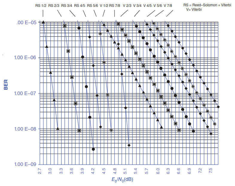
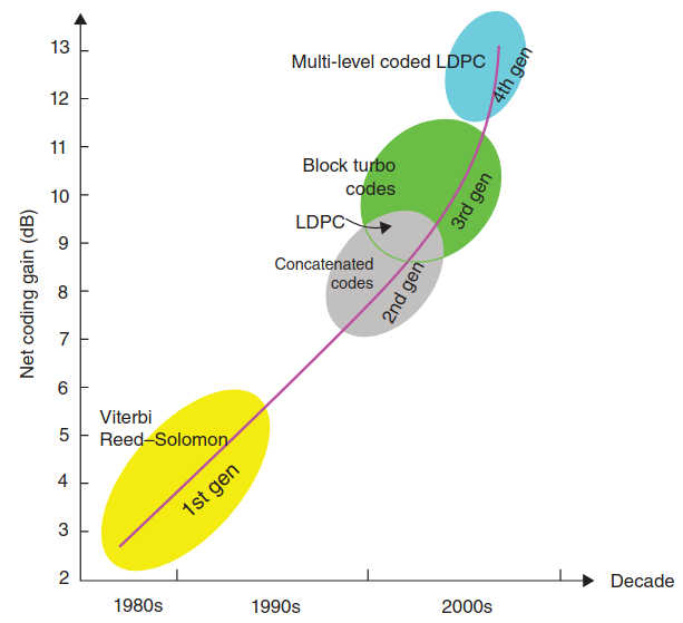
Research activities in FEC techniques in the past 20 years have given rise to new theoretical approaches. Modern approaches are parallel or serially concatenated convolutional codes, product codes, and low-density parity check codes (LDPCs) – all of which use “turbo” (i. e., recursive) decoding techniques. Satellite modems intended for common use during the past decade have employed “RS + Viterbi” encoding extensively; newer systems use either Turbo Codes or LDPC. Figure 5 shows the progression of the work in the recent past.
In looking at a diagram that plots BER versus Eb/No, we can find that there typically is an initial steep reduction in error probability as Eb/No increases (this area is called the waterfall region), followed by a region of shallower reduction (this is called the error floor region).
Improvements have occurred in recent years. In the late 1960s, Forney introduced a concatenated scheme of inner and outer FEC codes: the inner code is decoded using soft-decision channel information, while the outer Reed–Solomon code uses errors and erasures. In 1993, a new coding and decoding scheme was reported that achieves near-capacity performance on additive white Gaussian noise channel. The technique was dubbed “Turbo codes” by its discoverers. It is based in the use of two concatenated convolutional codes in parallel. The turbo code has a floor error near 10−5 , but the design of the interleaver is very critical in order to achieve good results in low BER (it is possible to avoid the floor error with an adequate design of the interleaver).
In 1996, a new technique was proposed, based in the same idea of Turbo codes, called Serial Concatenated Convolutional Codes (SCCCs); this new codification technique achieves better results for low BER than Turbo code.
This technique avoids both problems of Turbo codes:
- First, the floor error disappears, and;
- Second, the design of the interleaver is easier, because the input data of the two encoders are different.
After the introduction of Turbo codes. one has seen the emergence of a plethora of codes that exploit a Turbo-like structure. The common aspect of all Turbo-like codes (TLCs) is the concatenation of two or more simple codes separated by an interleaver, combined with an iterative decoding strategy.
TLC algorithms are:
- Parallel Concatenated Convolutional Codes (PCCCs) (this is the classical Turbo code);
- SCCCs;
- LDPC, and;
- Turbo Product Codes (TPCs).
Turbo codes and TLC offer good coding gain compared to traditional FEC approaches – as much as 3 dB in many cases. The area where TLCs have traditionally excelled is in the waterfall region – there are TLCs that are within a small fraction of a dB of the Shannon limit in this region; however, many TLCs have an almost flat error floor region, or one that starts at a very high error rate, or both.
This means that the coding gain of these TLCs rapidly diminishes as the target error rate is reduced. The performance of a TLC in the error floor region depends on several factors, such as the constituent code design and the interleaver design, as noted, but it typically worsens as the code rate increases or the block size decreases. Many TLC designs perform well only at high error rates, low code rates, or large block sizes; furthermore, these designs often target only a single code rate, block size, and modulation scheme, or suffer degraded performance or increased complexity to achieve flexibility in these areas.
Read also: Empowering Global Communication with INMARSAT Satellites in shipping
Parallel Concatenated Convolutional Codes (PCCC). PCCCs consist of the parallel concatenation of two convolutional codes. One encoder is fed the block of information bits directly, while the other encoder is fed an interleaved version of the information bits. The encoded outputs of the two encoders must be mapped to the signal set used on the channel. A PCCC encoder is formed by two (or more) constituent systematic encoders joined through one or more interleavers. The input information bits feed the first encoder and, after having been scrambled by the interleaver, they enter the second encoder. A code word of a parallel concatenated code consists of the input bits to the first encoder followed by the parity check bits of both encoders.
PCCC achieves near-Shannon-limit error correction performance. Bit error probabilities as low as 10-5 at Eb/No = 0,6 dB have been shown. PCCCs yield very large coding gains (10 or 11 dB) at the expense of a small data reduction or BW increase (Table 2).
| Table 2. Key Aspects of Various Turbo Codes | |
|---|---|
| Coding Type | Characteristics |
| Parallel concatenated convolutional codes (PCCC) | Good threshold performance – Among the best threshold performance of all TLCs. |
| Poor floor performance – The worst floor performance of all TLCs. With 8-state constituent codes BER floors are typically in the range 10-6–10-8, but this can be reduced to the 10-8–10-10 range by using 16-state constituent codes. However, achieving floors below 10-10 is difficult, particularly for high code rates and/or small block sizes. There are PCCC variants that have improved floors, such as concatenating more than two constituent codes, but only at the expense of increased complexity. | |
| High complexity code constraints – With 8- or 16-state constituent codes, the PCCC decoder complexity is rather high. | |
| Fast convergence – Among the best convergence of all TLCs. Typically, only 4–8 iterations are required. | |
| Fair code rate flexibility – Code rate flexibility is easily achieved by puncturing the outputs of the constituent codes. However, for very high code rates the amount of puncturing required is rather high, which degrades performance and increases decoder complexity (particularly with windowed decoding algorithms). | |
| Good block size flexibility – The block size is easily modified by changing the size of the interleaver, and there exist many flexible interleaver algorithms that achieve good performance. | |
| Good modulation flexibility – The systematic bits and the parity bits from each constituent code must be combined and mapped to the signal set. | |
| Serially concatenated convolutional codes (SCCC) | Medium threshold performance – The threshold performance of SCCCs is typically 0,3 dB worse than PCCCs. |
| Good floor performance – Among the best floor performance of all TLCs. Possible to have BER floors in the range 10-8–10-10 with 4-state constituent codes, and below 10-10 with 8-state constituent codes. However, floor performance is degraded with high code rates. | |
| Medium complexity code constraints – Code complexity constraints are typically low, but are higher for high code rates. Also, constituent decoder complexity is higher than for the equivalent code in a PCCC because soft decisions of both systematic and parity bits must be formed. | |
| Fast convergence – Convergence is even faster than PCCCs, with typically 4–6 iterations required. | |
| Poor code rate flexibility – As for PCCCs, code rate flexibility is achieved by puncturing the outputs of the constituent encoders. However, because of the serial concatenation, this puncturing must be higher for SCCCs than for PCCCs for an equivalent overall code rate. | |
| Good block size flexibility – As for PCCCs, block size flexibility is achieved simply by changing the size of the interleaver. However, for equivalent information block sizes the interleaver of an SCCC is larger than for a PCCC, so there is a complexity penalty in SCCCs for large block sizes. Also, if the code rate is adjusted by puncturing the outer code, then the interleaver size will depend on both the code rate and block size, which complicates reconfigurability. | |
| Very good modulation flexibility – As the inner code on an SCCC is connected directly to the channel, it is relatively simple to map the bits onto the signal set. | |
| Low-density parity check codes (LDPC) | Good threshold performance – LDPCs have been reported that have threshold performance within a tiny fraction of a dB of the Shannon Limit. However, for practical decoders their threshold performance is usually comparable to that of PCCCs. |
| Medium floor performance – Floors are typically better than PCCCs, but worse than SCCCs. | |
| Low-complexity code constraints – LDPCs have the lowest complexity code constraints of all TLCs. However, high throughput LDPC decoders require large routing resources or inefficient memory architectures, which may dominate decoder complexity. Also, LPDC encoders are typically a lot more complex than other TLC encoders. | |
| Slow convergence – LDPC decoders have the slowest convergence of all TLCs. Many published results are for 100 iterations or more. However, practical LDPC decoders will typically use 20–30 iterations. | |
| Good code rate flexibility – LDPCs can achieve good code rate flexibility. | |
| Poor block size flexibility – For LDPCs to change block size, they must change their parity check matrix, which is quite difficult in a practical, high throughput decoder. | |
| Good modulation flexibility – As with PCCCs the output bits of an LDPC must be mapped onto the signal sets of different modulation schemes. | |
| Turbo product codes (TPC) | Poor threshold performance – TPCs have the worst threshold performance of all TLCs; they can have thresholds that are as much as 1 dB worse than PCCCs. However, for very high code rates (0,95 and above) they will typically outperform other TLCs. |
| Medium floor performance – Their floors are typically lower than PCCC, but not as low as SCCC. | |
| Low-complexity code constraints – TPC decoders have the lowest complexity of all TLCs, and high throughput parallel decoders can readily be constructed. | |
| Medium convergence – TPC decoders converge quickly, with 8–16 iterations being typically required. | |
| Poor rate flexibility – The overall rate of a TPC is dictated by the rate of its constituent codes. There is some flexibility available in these rates, but it is difficult to choose an arbitrary rate. | |
| Poor block size flexibility – The overall block size of a TPC is dictated by the block size of its constituent codes. It is difficult to choose an arbitrary block size, and especially difficult to choose an arbitrary code rate and an arbitrary block size. | |
| Good modulation flexibility – As with PCCCs and LDPCs, the output bits must be mapped onto the signal sets. | |
Serially Concatenated Convolutional Codes (SCCC). SCCCs consist of the serial concatenation of two convolutional codes. The outer encoder is fed the block of information bits and its encoded output is interleaved before being input to the inner encoder. The encoded outputs of only the inner encoder must be mapped to the signal set used on the channel. A code word of a serial concatenated code consists of the input bits to the first encoder followed by the parity check bits of both encoders. SCCC achieves near-Shannon-limit error correction performance. Bit error probabilities as low as 10-7 at Eb/No = 1 dB have been shown. SCCC yields very large coding gains (10 or 11 dB) at the expense of a small data reduction or BW increase (Table 2).
Low-Density Parity Check Codes (LDPC). LDPCs are block codes defined by a sparse parity check matrix. This sparseness admits a low-complexity iterative decoding algorithm. The generator matrix corresponding to this parity check matrix can be determined and used to encode a block of information bits; these encoded bits must then be mapped to the signal set used on the channel. The performance of LDPC is within 1 dB of the theoretical maximum performance known as the Shannon limit (Table 2).
Turbo Product Codes (TPC). In a TPC system the information bits are arranged as an array of equal-length rows and equal-length columns. The rows are encoded by one block code and then the columns (including the parity bits generated by the first encoding) are encoded by a second block code. The encoded bits must then be mapped onto the signal set of the channel (Table 2).
Filters and Roll-Off Factors
Newer modulation techniques utilize tighter roll-off factors. Some basic concepts related to roll-off and filters are provided in this section. High symbol rate modulation may give rise to (undesirable) signals in bands other than the assigned/intended band. Occupied BW is a measure of how much frequency spectrum is covered by the signal in question; the units are in Hertz, and measurement of occupied BW generally implies a power percentage or ratio. A typical direct conversion transmitter uses the low-pass filters (LPFs) to eliminate out-of-band signal components from the baseband signal, but these components may re-appear along the way as a result of intermodulation distortion generated within the transmitter, for example, in the downstream power amplifier (PA), such as the satellite transponder.
This tendency to regain undesirable signal components is called “spectral regrowth.” Adjacent Channel Power Ratio (ACPR) is a popular measure of spectral regrowth in digital transmitters and is often a design specification. Nonlinearities in the transmitter introduce harmonics of ωm about the carrier fundamental. Given these observations on the possibility for spectral regrowth, a key question is whether a modulated signal fits “neatly” inside a transponder, or whether there may be a leakage of signal into another transponder.
Figure 6 depicts the relative power spectral density (in W/Hz, measured in dB) of a digitally modulated carrier that uses BPSK and QPSK without applying any filtering (the x-axis shows normalized frequency (f-fc)/(bit rate) where fc is the carrier frequency; the y-axis is the relative level of the power density with respect to the maximum value at carrier frequency fc).
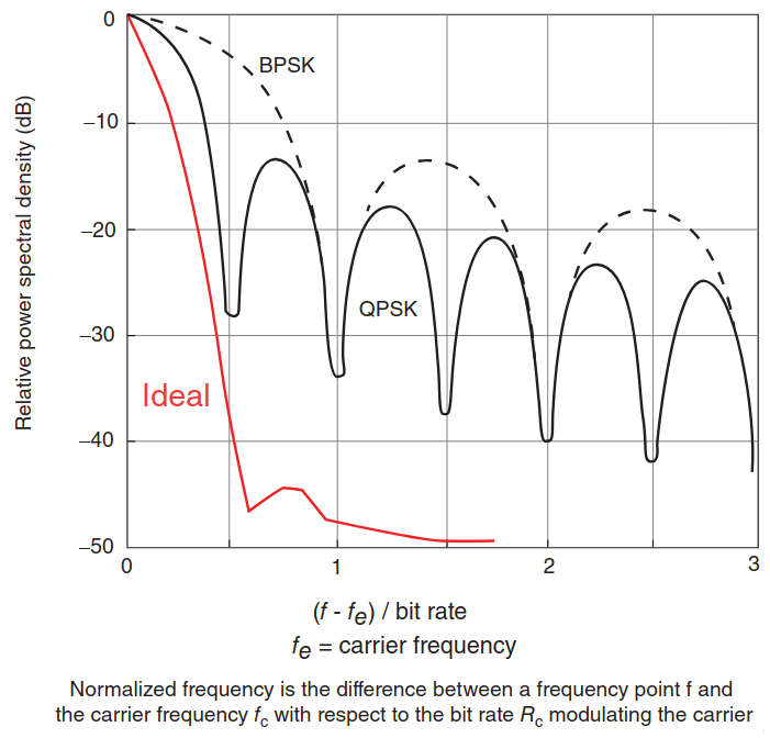
Two issues are worth considering:
- The width of the principal lobe of the spectrum of the modulated signal, which affects the required/utilized BW of the channel, and;
- The secondary sidelobes, which affect adjacent carriers by generating interference when the spectral decay with respect to frequency is not as sharp as one would hope.
The figure shows that QPSK is “better” than BPSK, having a lower main lobe. This is because, in general, constellation diagrams show that transition to new states could result in large amplitude changes (e. g., going from 010 to 110 in 8-PSK), and a signal that changes amplitude over a very large range will exercise amplifier non-linearities, which cause distortion products. In continuously modulated systems large signal changes will cause “spectral regrowth” or wider modulation sidebands (a phenomenon related to intermodulation distortion).
The problem lies in nonlinearities in the circuits. If the amplifier and associated circuits were perfectly linear, the spectrum (spectral occupancy or occupied BW) would be unchanged. As stated, any fast transition in a signal, whether in amplitude, phase, or frequency, results in a power-frequency spectrum that requires a wide occupied BW. Any technique that helps to slow down transitions narrows the occupied BW. To deal with this spectral regrowth issue and limit unwanted interference to adjacent channels filtering is used at the transmitter side. In addition to the intrinsic phenomenon of spectral spreading of the modulation sidelobes, an attempt to transmit at maximum power, either at the remote terminal or at the satellite, produces amplitude and phase distortions. To avoid operating in the nonlinear region of the amplifier, one typically needs to backoff (from using) the maximum transponder power.
The rest of this section focuses on filtering. Filtering allows the transmitted BW to be reduced without losing the content of the digital data, thereby improving the spectral efficiency of the signal.
The most common filtering techniques are:
- raised cosine filters,
- square-root raised cosine filters,
- and Gaussian filters.
Filtering smoothes transitions (in I and Q), and, as a result, reduces interference because it reduces the tendency of one signal or one transmitter to interfere with another in a Frequency Division Multiple Access (FDMA) system. At the receiver’s end, reduced BW improves sensitivity because more noise and interference are rejected.
It should be noted, however, that some trade-offs must be taken into consideration:
- Carrier power cannot be limited (clipped) without causing the spectrum to spread out once again;
- Because narrowing the spectral occupancy was the reason the filtering was inserted in the first place;
- The designer must select the choice carefully.
One trade-off is that some types of filtering cause the trajectory of the signal (the path of transitions between the states) to overshoot in many cases. This overshoot can occur in certain types of filters (such as Nyquist filters). This overshoot path represents carrier power and phase. For the carrier to take on these values more output power from the transmitter amplifiers is required; specifically, it requires more power than would be necessary to transmit the actual symbol itself. Another consideration is Inter-Symbol Interference (ISI). ISI is the interference between adjacent symbols often caused by system filtering, dispersion in optical fibers, or multipath propagation in radio system. This occurs when the signal is filtered enough so that the symbols blur together and each symbol affects those around it. This is determined by the time-domain response or impulse response of the filter. There are different types of filtering.
As noted, the most common are The rest of this subsection is based on Reference.x:
- Raised cosine,
- Square-root raised cosine,
- and Gaussian filters.
Raised cosine filters are a class of Nyquist filters. Nyquist filters have the property that their impulse response rings That is, it has the impulse response of the filter cross through zero.x at the symbol rate. The time response of the filter goes through zero with a period that exactly corresponds to the symbol spacing. Adjacent symbols do not interfere with each other at the symbol times because the response equals zero at all symbol times, except the center (desired) one.
Nyquist filters filter the signal heavily without blurring the symbols together at the symbol times; this is important for transmitting information without errors caused by ISI. Note that ISI does exist at all times except the symbol (decision) times. Usually, the filter is split, half being in the transmit path and half in the receiver path; in this case root Nyquist filters (also commonly called root raised cosine) are used in each part, such that their combined response is that of a Nyquist filter. The raised cosine filter is an implementation of a low-pass Nyquist filter; its spectrum exhibits odd symmetry about 1/2T where T is the symbol period of the communications system.
The frequency-domain description of the raised cosine filter is a piecewise function characterized by two values: α, the roll-off factor, and T, specified as:
The roll-off factor, α, is a measure of the excess BW of the filter, that is, the BW occupied beyond the Nyquist BW of 1/2T.
If we denote the excess BW as Δf, then:
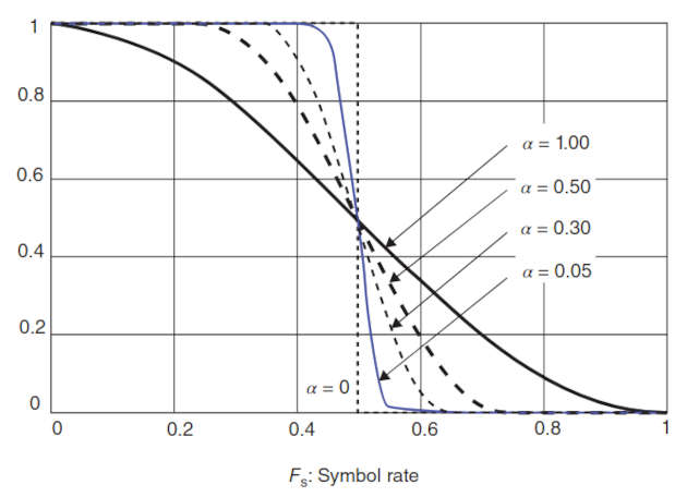
where Rs = 1/T and T the symbol period (symbol energy expands into the [−T, T] interval in a time-amplitude domain). The time-domain ripple level increases as decreases (from 0 to 1). The excess BW of the filter can be reduced, but only at the expense of an elongated impulse response. As α approaches 0, the roll-off zone becomes infinitesimally narrow; hence, the filter converges to an ideal or brick wall filter. When α = 1, the nonzero portion of the spectrum is a pure raised cosine.
The BW of a raised cosine filter is most commonly defined as the width of the nonzero portion of its spectrum, that is:
α is sometimes called the “excess BW factor” as it indicates the amount of occupied BW that will be required in the case of excessive, ideal occupied BW (which would be the same as the symbol rate).
The sharpness of a raised cosine filter is described by α (Figure 7).
α provides a measure of the occupied BW of the system:
with symbol rate = 1/2T = (1/2) Rs.
If the filter had a perfect (brick wall) characteristic with sharp transitions and α = 0, the occupied BW would be:
In a perfect world, the occupied BW would be the same as the symbol rate, but this is not practical. An α = 0 is impossible to implement. At the other extreme, consider a broader filter with an α = 1, which is easier to implement.
The occupied BW will be:
An α = 1 uses twice as much BW as an α = 0. In practice, it is possible to implement an α below 0,2 and make good, compact, practical devices, though some video systems use an α as low as 0,10. Typical values range from 0,35 to 0,5 The corresponding term for a Gaussian filter is BT (bandwidth time product). Occupied bandwidth cannot be stated in terms of BT because a Gaussian filter’s frequency response does not go identically to zero, as does a raised cosine. Common values for BT are 0,3–0,5.x.
A designer seeks to maximize the power and BW efficiency of satellite terminals, in particular, for Very Small Aperture Terminals (VSATs), where a key limitation to communication capacity is a nonlinear transmitting PA. It is highly undesirable to waste the RF spectrum by using channel bands that are too wide. Therefore, filters are used to reduce the occupied BW of the transmission. The data pulse stream is band-limited for BW efficiency; however, the effect of filtering (in the time domain) is to cause envelope excursions outside the linear region of the PA characteristic. The traditional approach is to reduce the average power at the input of the amplifier such that the maximum signal excursions are within the linear range of the amplifier characteristic. This reduction is termed power backoff and, as defined earlier, can be significant for BW-efficient systems.
Narrow filters with sufficient accuracy and repeatability are somewhat difficult to build. Smaller values of α increase ISI because more symbols can contribute to the demodulated signal; this tightens the requirements on clock accuracy. These narrower filters also result in more overshoot and, therefore, more peak carrier power. The PA must then accommodate the higher peak power without distortion. Larger amplifiers cause more heat and thus cause more electrical interference to be produced because the RF current in the PA will interfere with other circuits.
Predistortion methods in the uplink station can be used to minimize the effect of transponder nonlinearity. As shown in table below, PAs are inherently nonlinear and when operated near saturation cause intermodulation products that interfere with adjacent and alternate channels. This interference affects the adjacent channel leakage ratio (ACLR).
| Partial Listing of System-Level us Patents for Spot-Beam/Multi-Beam Satellites | ||||
|---|---|---|---|---|
| Patent | Filing Date | Publication Date | Applicant | Title |
| US3810255 | Jun 10, 1971 | May 7, 1974 | Communications Satellite Corporation | Frequency translation routing communications transponder |
| US4228401 | Dec 22, 1977 | Oct 14, 1980 | Communications Satellite Corporation | Communication satellite transponder interconnection utilizing variable bandpass filter |
| US4689625 | Nov 6, 1984 | Aug 25, 1987 | Martin Marietta Corporation | Satellite communications system and method therefor |
| US4813036 | Nov 27, 1985 | Mar 14, 1989 | National Exchange, Incorporated | Fully interconnected spot beam satellite communication system |
| US4706239 | Dec 18, 1985 | Nov 10, 1987 | Kokusai Denshin Denwa Company, Limited | Communications satellite repeater |
| US4858225 | Nov 5, 1987 | Aug 15, 1989 | International Telecommunications Satellite | Variable bandwidth variable center-frequency multibeam satellite-switched router |
| US4931802 | Mar 11, 1988 | Jun 5, 1990 | Communications Satellite Corporation | Multiple spot-beam systems for satellite communications |
| US5119225 | Jan 18, 1989 | Jun 2, 1992 | British Aerospace Public Limited Company | Multiple access communication system |
| US4903126 | Feb 10, 1989 | Feb 20, 1990 | Kassatly Salim A | Method and apparatus for TV broadcasting |
| US5394560 | Sep 30, 1992 | Feb 28, 1995 | Motorola, Incorporated | Nationwide satellite message delivery system |
| US5428814 | Aug 13, 1993 | Jun 27, 1995 | Alcatel Espace | Space communications apparatus employing switchable band filters for transparently switching signals on board a communications satellite, payload architectures using such apparatus, and methods of implementing the apparatus and the architectures |
| US5412660 | Sep 10, 1993 | May 2, 1995 | Trimble Navigation Limited | ISDN-to-ISDN communication via satellite microwave radio frequency communications link |
| US5424862 | Apr 28, 1994 | Jun 13, 1995 | Glynn; Thomas W | High capacity communications satellite |
| US5594780 | Jun 2, 1995 | Jan 14, 1997 | Space Systems/Loral, Incorporated | Satellite communication system that is coupled to a terrestrial communication network and method |
| US5640386 | Jun 6, 1995 | Jun 17, 1997 | Globalstar L.P. | Two-system protocol conversion transceiver repeater |
| US5552920 | Jun 7, 1995 | Sep 3, 1996 | Glynn; Thomas W | Optically crosslinked communication system (OCCS) |
| US5680240 | Jun 12, 1995 | Oct 21, 1997 | Glynn; Thomas W | High capacity communications satellite |
| EP0748064A2 | Apr 3, 1996 | Dec 11, 1996 | Globalstar L.P | Two-system protocol conversion transceiver repeater |
| US5822312 | Apr 17, 1996 | Oct 13, 1998 | Com Dev Limited | Repeaters for multibeam satellites |
| US5809141 | Jul 30, 1996 | Sep 15, 1998 | Ericsson Incorporated | Method and apparatus for enabling mobile-to-mobile calls in a communication system |
| US5898681 | Sep 30, 1996 | Apr 27, 1999 | Amse Subsidiary Corporation | Methods of load balancing and controlling congestion in a combined frequency division and time division multiple access communication system using intelligent login procedures and mobile terminal move commands |
| US5963862 | Oct 25, 1996 | Oct 5, 1999 | Pt Pasifik Satelit Nusantara | Integrated telecommunications system providing fixed and mobile satellite-based services |
| US5864546 | Nov 5, 1996 | Jan 26, 1999 | Worldspace International Network, Incorporated | System for formatting broadcast data for satellite transmission and radio reception |
| US5697050 | Dec 12, 1996 | Dec 9, 1997 | Globalstar L.P | Satellite beam steering reference using terrestrial beam steering terminals |
| US6256496 | Mar 10, 1997 | Jul 3, 2001 | Deutsche Telekom Ag | Digital radio communication apparatus and method for communication in a satellite-supported VSAT network |
| US5884142 | Apr 15, 1997 | Mar 16, 1999 | Globalstar L.P | Low earth orbit distributed gateway communication system |
| EP0883252A2 | May 30, 1998 | Dec 9, 1998 | Hughes Electronics Corporation | Method and system for providing wideband communications to mobile users in a satellite-based network |
| US6278876 | Jul 13, 1998 | Aug 21, 2001 | Hughes Electronics Corporation | System and method for implementing terminal to terminal connections via a geosynchronous earth orbit satellite |
| US6496682 | Sep 14, 1998 | Dec 17, 2002 | Space Systems/Loral, Incorporated | Satellite communication system employing unique spot beam antenna design |
| US6415329 | Oct 30, 1998 | Jul 2, 2002 | Massachusetts Institute of Technology | Method and apparatus for improving efficiency of TCP/IP protocol over high delay-bandwidth network |
| EP0967745A2 | Jun 23, 1999 | Dec 29, 1999 | Matsushita Electric Industrial Co., Limited | Receiving apparatus for receiving a plurality of digital transmissions comprising a plurality of receivers |
| US6240124 | Nov 2, 1999 | May 29, 2001 | Globalstar L.P | Closed loop power control for low earth orbit satellite communications system |
| US7245933 | Mar 1, 2000 | Jul 17, 2007 | Motorola, Incorporated | Method and apparatus for multicasting in a wireless communication system |
| US7068616 | Apr 20, 2001 | Jun 27, 2006 | The Directv Group, Incorporated | Multiple dynamic connectivity for satellite communications systems |
| US7809403 | May 15, 2001 | Oct 5, 2010 | The Directv Group, Incorporated | Stratospheric platforms communication system using adaptive antennas |
| US20030109220 | Dec 12, 2001 | Jun 12, 2003 | Hadinger Peter J | Communication satellite adaptable links with a ground-based wideband network |
| US6965755 | Nov 8, 2002 | Nov 15, 2005 | The Directv Group, Incorporated | Comprehensive network monitoring at broadcast satellite sites located outside of the broadcast service area |
| US7069036 | Feb 13, 2003 | Jun 27, 2006 | The Boeing Company | System and method for minimizing interference in a spot beam communication |
| US7715838 | Apr 2, 2003 | May 11, 2010 | The Boeing Company | Aircraft based cellular system |
| US7653349 | Jun 18, 2003 | Jan 26, 2010 | The DirecTV Group, Incorporated | Adaptive return link for two-way satellite communication systems |
| US8358971 | Jun 23, 2003 | Jan 22, 2013 | Qualcomm Incorporated | Satellite-based programmable allocation of bandwidth for forward and return links |
| US7525934 | Sep 13, 2004 | Apr 28, 2009 | Qualcomm Incorporated | Mixed reuse of feeder link and user link bandwidth |
| US7580708 | Sep 8, 2005 | Aug 25, 2009 | The DirecTV Group, Incorporated | Comprehensive network monitoring at broadcast satellite sites located outside of the broadcast service area |
| US7636546 | Dec 20, 2005 | Dec 22, 2009 | Atc Technologies, Llc | Satellite communications systems and methods using diverse polarizations |
| WO2006123064A1 | May 19, 2006 | Nov 23, 2006 | Centre Nat Etd Spatiales | Method for assigning frequency subbands to upstream radiofrequency connections and a network for carrying out said method |
| US7962134 | Jan 17, 2007 | Jun 14, 2011 | MNC Microsat Networks (Cyprus) Limited | Systems and methods for communicating with satellites via non-compliant antennas |
| US8078141 | Jan 17, 2007 | Dec 13, 2011 | Overhorizon (Cyprus) Plc | Systems and methods for collecting and processing satellite communications network usage information |
| US8326217 | Jan 17, 2007 | Dec 4, 2012 | Overhorizon (Cyprus) Plc | Systems and methods for satellite communications with mobile terrestrial terminals |
| US20090191810 | May 15, 2007 | Jul 30, 2009 | Mitsubishi Electric Corporation | Satellite communication system |
| US8346161 | May 15, 2007 | Jan 1, 2013 | Mitsubishi Electric Corporation | Satellite communication system |
| US8050628 | Jul 17, 2007 | Nov 1, 2011 | MNC Microsat Networks (Cyprus) Limited | Systems and methods for mitigating radio relay link interference in mobile satellite communications |
| US7869759 | Dec 12, 2007 | Jan 11, 2011 | Viasat, Incorporated | Satellite communication system and method with asymmetric feeder and service frequency bands |
| US8311498 | Sep 29, 2008 | Nov 13, 2012 | Broadcom Corporation | Multiband communication device for use with a mesh network and methods for use therewith |
| US20090291633 | Mar 18, 2009 | Nov 26, 2009 | Viasat, Incorporated | Frequency re-use for service and gateway beams |
| US20090298416 | Mar 18, 2009 | Dec 3, 2009 | Viasat, Incorporated | Satellite Architecture |
| US20120276840 | Mar 18, 2009 | Nov 1, 2012 | Viasat, Incorporated | Satellite Architecture |
| US8254832 | Mar 18, 2009 | Aug 28, 2012 | Viasat, Incorportated | Frequency re-use for service and gateway beams |
| US8315199 | Mar 18, 2009 | Nov 20, 2012 | Viasat, Incorporated | Adaptive use of satellite uplink bands |
| US8538323 | Mar 18, 2009 | Sep 17, 2013 | Viasat, Incorporated | Satellite architecture |
| US8339309 | Sep 24, 2010 | Dec 25, 2012 | Mccandliss Brian | Global communication system |
| US20120164941 | Dec 16, 2011 | Jun 28, 2012 | Electronics and Telecommunications Research Institute | Beam bandwidth allocation apparatus and method for use in multi-spot beam satellite system |
| US20120244798 | May 30, 2012 | Sep 27, 2012 | Viasat, Incorporated | Frequency re-use for service and gateway beams |
| US8548377 | May 30, 2012 | Oct 1, 2013 | Viasat, Incorporated | Frequency re-use for service and gateway beams |
Linearization techniques allow PAs to operate efficiently and at the same time maintain acceptable ACLR levels (in effect, linearization affords the use of a lower-cost more efficient PA in place of a higher-cost less-efficient PA). PAs in the field today are predominately linearized by some form of feed-forward technology.
In recent years, however, designers have stated to employ digital predistortion (also known as preemphasis); compared to feed-forward architectures, designs based on digital predistortion approaches enjoy higher efficiency at lower cost. Predistortion is a system process designed to increase, within a band of frequencies, the magnitude of some (usually higher) frequencies with respect to the magnitude of other (usually lower) frequencies, in order to improve the overall SNR by minimizing the adverse effects of such phenomena as attenuation differences, or saturation of the PA. In a group of waves that have slightly different individual frequencies, the group delay time is defined as the time required for any defined point on the envelope (i. e., the envelope determined by the additive resultant of the group of waves) to travel through a device or transmission facility.
Group delay is thus the rate of change of the total phase shift with respect to angular frequency, dθ/dω, through a device or transmission medium, where θ the total phase shift can be found, ω the angular frequency is equal to 2πsf, and f is the frequency. Predistortion can be employed to deal with group delay.
DVB-S2 and DVB-S2 Extensions
Because of the nature of the satellite link (noise, attenuation), 8-PSK is the traditional technical “sweet spot”; however, more complex modulation schemes are being introduced.
It should be noted that it is useful to employ standards to deploy systems so that equipment from multiple suppliers can be used in a large network (although generally for a variety of other reasons – particularly network management – operators tend not to comingle equipment for the same element of an RF link in any large measure).
DVB-S2 Modulation
DVB-S2 is a second-generation framing structure, channel coding and modulation system for broadcasting, interactive services, news gathering and other broadband satellite applications. DVB-S2 is a specification developed by the Digital Video Broadcasting (DVB) Project adopted by European Telecommunications Standards Institute (ETSI) standards is now used worldwide. As the name implies, DVB-S2 is second-generation specification for satellite broadcasting; it was developed in 2003. Extensions were being proposed and standardized at press time. This section discusses DVB-S2 (see below) followed by an analysis of extensions, which build on and extend DVB-S2 (see below).
The DVB-S2 standard has been specified with the goals of:
- Achieving best transmission performance;
- Embodying flexibility, and;
- Requiring reasonably low receiver complexity (using existing chip technology).
The basic documents defining the DVB-S2 standard are:
- ETSI: Draft EN 302 307: DVB; Second generation framing structure, channel coding and modulation systems for Broadcasting, Interactive Services, News Gathering and other broadband satellite applications (DVB-S2).
- EN302307v1.1.1 in 2005-03;
- EN302307v1.1.2 in 2006-06;
- EN302307v1.2.1 in 2009-08;
- EN302307v1.3.1 in 2013-03.
- ETSI: EN 300 421: DVB; Framing structure, channel coding and modulation for 11/12 GHz satellite services;
- ETSI: EN 301 210: DVB: Framing structure, channel coding and modulation for Digital Satellite News Gathering (DSNG) and other contribution applications by satellite.
The DVB-S2 system has been designed for satellite broadband applications such as broadcast services for MPEG-2/MPEG-4 Standard Definition Television (SDTV) and High Definition Television (HDTV) (including single or multiple MPEG Transport Streams (TSs), continuous bit streams, and IP packets), and interactive services, namely, Internet access. The DVB-S2 system may be used in “single-carrier-per-transponder” or in “multi-carriers-per-transponder” configurations. When introduced in the 2000s, the DVB-S2 standard was a quantum leap in terms of BW efficiency compared to the former DVB-S and DVB-DSNG standards.
This improvement is not only because of the use of LDPC for FEC, but also of new modulation schemes and new modes of operations, specifically, Variable Coding and Modulation (VCM) and Adaptive Coding and Modulation (ACM). AMC is a link adaptation method (typically used in 3G mobile wireless communications) that provides the flexibility to match the modulation-coding scheme to the average channel conditions for each user.
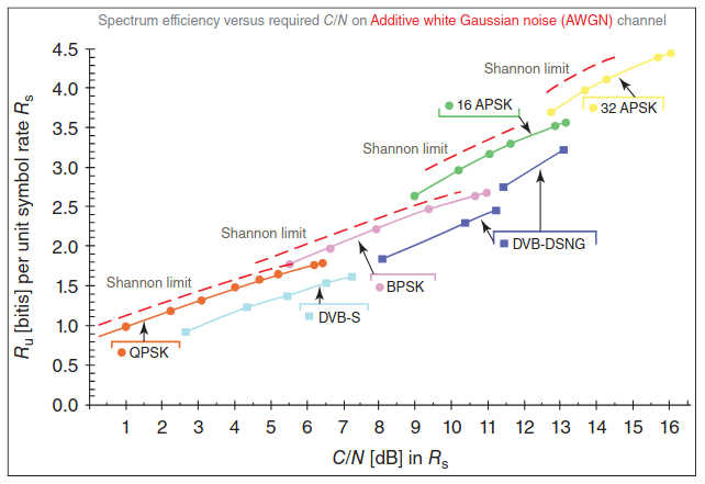
When using AMC, the modulation and coding format is changed dynamically to match the current-received signal quality or channel conditions (however, the power of the transmitted signal is held constant over a frame interval). A DVB-S2 system can operate at C/N from -2,4 dB (using QPSK with FEC at 1/4 rate) to 16 dB (using 32-APSK with FEC at 9/10 rate), assuming an Additive White Gaussian Noise (AWGN) channel and ideal demodulator. The distance from the Shannon limit ranges from 0,7 to 1,2 dB. On AWGN, the result is typically a 20–35 % capacity increase over DVB-S and DVB-DSNG under the same transmission conditions and 2–2,5 dB more robust reception for the same spectrum efficiency.
DVB-S is the original DVB specification for satellite-based television distribution; DVB-S was standardized in 1994. The broadcast industry adopted the format in the late 1990s because it established a universal framework for MPEG-2 based digital television services to be broadcast over satellite using Viterbi concatenated with RS (Viterbi + RS) FEC and QPSK modulation. The performance of this code is such that a coding rate of at least 2/3 QPSK is required (to achieve a BER < 10-7); a typical Eb/No of 6,5 dB is needed. The actual (payload) bit rate for 30 Mbaud with QPSK 2/3 is 1,229 · 30 = 36,87 Mbps. In 1999, the DVB-S standard was extended and became the DVB-DSNG standard. This new standard allowed for more efficient modes of modulation (such as 8-PSK and 16-QAM) to be utilized. Introducing the higher-order modulation resulted in overall savings in BW and required an increase of power to achieve similar Eb/No results.
We discuss DVB-S2 (and DVB-S) features briefly herewith to counterpoint these features with the capabilities of DVB-S2X. As noted above, to achieve the optimal performance complexity trade-off (about 30 % capacity gain over DVB-S), DVB-S2 makes use of recent advancements in channel coding and modulation. Specifically, DVB-S2 uses LDPC concatenated with BCH coding. The chosen LDPC FEC codes utilize large blocks (64 800 bits for applications not too critical for delays, and 16 200 bits for application that are more critical).
Code rates 1/4, 1/3, 2/5, 1/2, 3/5, 2/3, 3/4, 4/5, 5/6, 8/9, and 9/10 are available, depending on the selected modulation and the system requirements. Coding rates 1/4, 1/3, and 2/5 have been introduced to operate, in combination with QPSK, under poor link conditions, where the signal level is below the noise level. Four modulation modes can be selected for the transmitted payload as shown in Figure 8:
- QPSK,
- 8-PSK,
- 16-APSK,
- and 32-APSK.
QPSK and 8-PSK are used for broadcast applications and can be used in nonlinear satellite transponders driven near saturation. While the 8-PSK scheme has seen extensive implementation and deployment, the 16-APSK and 32-APSK modes have been targeted at professional applications (they can also be used for broadcasting); these modulation schemes require a higher level of available C/N and the adoption of advanced predistortion methods in the uplink station to minimize the effect of transponder nonlinearity.
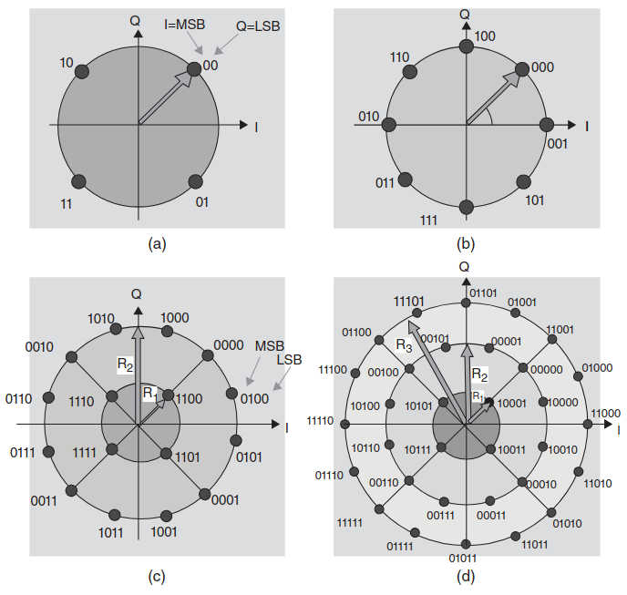
Although these modes are not as power efficient as the other modes, the spectrum efficiency is greater. The 16-APSK and 32-APSK constellations have been optimized to operate over a nonlinear transponder by placing the points on circles. Nevertheless, their performance on a linear channel is comparable with those of 16-QAM and 32-QAM, respectively. By selecting the modulation constellation and code rates, spectrum efficiencies from 0,5 to 4,5 bit per symbol become available and can be chosen on the basis of the capabilities and restrictions of the satellite transponder used. It should be noted that, in general, DVB-S2 is optimized for nonlinear operations [e. g., for Direct to Home (DTH) applications].
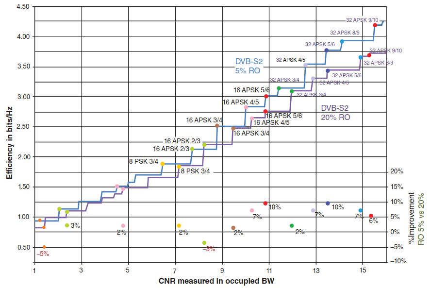
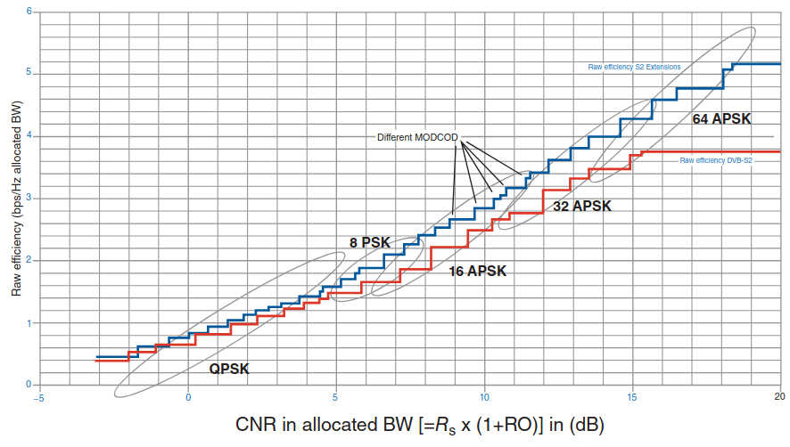
Figure 9 depicts these efficiencies for the modulation schemes supported. DVB-S2 has three “roll-off factor” choices to determine spectrum shape:
- 0,35 as in DVB-S, and;
- 0,25 and 0,20 for tighter BW restrictions (the use of the narrower roll-off α = 0,25 and α = 0,20 allows transmission capacity to increase, but may also produce larger nonlinear degradations by satellite for single-carrier operation).
As seen above, DVB-S2 standard allows up to 5 bits per symbol with a 32-APSK constellation.
Constant Coding Modulation (CCM) is the simplest mode of DVB-S2; it is similar to the DVB-S, in the sense that all data frames are modulated and coded using the same fixed parameters. The LDPC code has a performance such that a coding rate of 4/5 is sufficient for the same channel conditions. For example, a minimum Es/No of 5,4 dB supports QPSK 4/5. The useful bit rate is then given by 30 Mbaud × 1,587 = 47,61 Mbps. Compared to DVB-S, this is an efficiency improvement of around 30 %. This represents a 2–3 dB improvement compared to DVB-S.
Figure 10 compares DVB-S and DVB-S2 performance for QPSK and 8-PSK modulations with a variety of FEC rates.
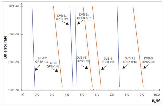
When one compares 8-PSK 2/3 FEC rate for a 1 · 10-9 bit error rate, the required Eb/No level for DVB-S is 6,10 dB versus 4,35 dB for DVB-S2, equating to a 1,75 dB reduction in the required power for the same Eb/No, reducing the required spectral power by 28,7 %. For a data rate of 6 Mbps using 8-PSK 2/3 FEC rate, the DVB-S would have a symbol rate of 3,26 Msps, assuming a carrier spacing factor of 1,3, and would require 4,23 MHz of BW on the satellite. In comparison, the DVB-S2 would have a symbol rate of 3,03 Msps requiring 3,94 MHz of BW on the satellite, resulting in a BW savings of approximately 6,9 %.
A feature of the DVB-S2 standard is that different services can be transmitted on the same carrier, each using their own modulation scheme and coding rate (Figure 11).
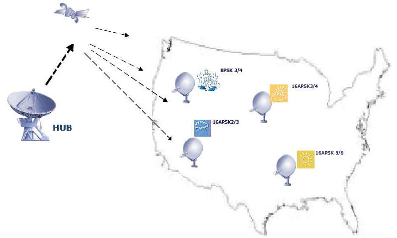
This “multiplexing” at the physical layer is known as VCM. VCM is useful when different services do not need the same protection level or different services are intended for different stations with different average receiving conditions. Using VCM, different Coding/Modulation (CM) mechanisms (also known as MODCODs) can be selected for each station. Typically, these CMs range between QPSK 4/5 and 16-APSK 2/3. If the total baud rate (30 Mbaud) is distributed equally over each station, each station will use a 30/20 = 1,5 Mbaud part of the carrier (assuming there were 20 stations in the system). The corresponding bit rates vary between 2,38 and 3,96 Mbps according to the selected CM.
The total available rate is then 61,09 Mbps. This is an improvement of around 65 % compared to DVB-S. When a return channel is available from each receiving site to the transmit site, DVB-S2 offers an even more versatile feature known as ACM. With ACM, it is possible to dynamically modify the coding rate and modulation scheme for every single frame, according to the measured channel conditions where the frame must be received. The return channel is used to dynamically report the receiving conditions at each receiving site. In this scenario, the CMs range between 8-PSK 3/4 and 16-PSK 5/6. If distributed equally over each station, each station will use a 30/20 = 1,5 Mbaud part of the carrier (assuming there were 20 stations in the system). The corresponding bit rates vary between 3,34 and 4,95 Mbps to each site. The total available rate is then 86,3 Mbps. This is more than 130 % higher than DVB-S.
To address a transition from DVB-S to DVB-S2, optional backward-compatible modes have been defined in DVB-S2. These modes allow one to send two TSs on a single satellite channel. The first (High Priority, HP) stream is compatible with DVB-S receivers as well as with DVB-S2 receivers, while the second (Low Priority, LP) stream is compatible with DVB-S2 receivers only.
When DVB-S2 is transmitted by satellite, quasi-constant envelope modulations such as QPSK and 8-PSK are power efficient in the single-carrier-per-transponder configuration, because they can operate on transponders driven near saturation. 16-APSK and 32-APSK, which are inherently more sensitive to nonlinear distortions and would require quasi-linear transponders [i. e., with larger Output Back Off (OBO)], may be improved in terms of power efficiency by using nonlinear compensation techniques in the uplink station. In FDM configurations, where multiple carriers occupy the same transponder, the latter must be kept in the quasi-linear operating region (i. e., with large OBO) to avoid excessive intermodulation interference between signals.
DVB-S2 Extensions
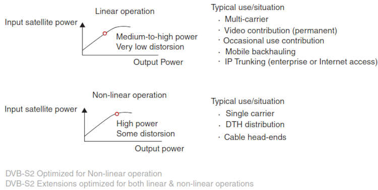
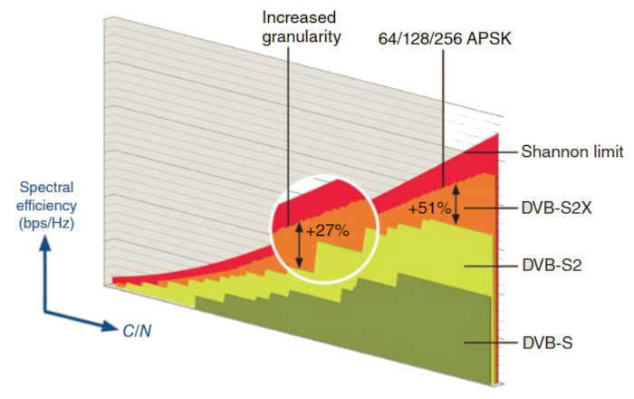
During Services, service options, and service providers change over time (new ones are added and existing ones may drop out as time goes by); as such, any service, service option, or service provider mentioned in this article is mentioned strictly as illustrative and possible examples of emerging technologies, trends, or approaches. As such, the intention is to provide pedagogical value. No recommendations are implicitly or explicitly implied by the mention of any vendor or any product (or lack thereof).x the past few years, work has been underway to further enhance the capabilities of DVB-S2. As mentioned already, higher throughput is needed for evolving applications such as Ultra HD and commercial aeronautical Internet access. Technical work was being wrapped up in 2014, and the expectation was that the new standard would be adopted; most likely it will be published as Annex to the DVB-S2 standard. On February 27, 2014, the DVB steering committee approved the specifications for the new standard, to be called DVB-S2X. DVB-S2X is a superset of DVB-S2. The Es/No range extends from –10 dB to +24 dB. DVB-S2X provides increased availability. While DVB-S2 is optimized for nonlinear operations, DVB-S2X handles both environments equally well (Figure 12).
DVB-S2X allows increased granularity in MODCODs and higher-order modulation schemes (e. g., 64-APSK). This allows one to achieve up to 37 % gain in spectral efficiency; also, generally, there are gains at lower MODCODs. Figure 13 depicts, in general terms, the relative improvements of the extensions. Compared with existing commercial implementations, the combination of technologies incorporated in the new standard results in a gain of up to 20 % for DTH networks and 51 % for other professional applications compared to DVB-S2 [WIL201401].
Modulation improvements are because of the ability to do more processing (continued advancements under “Moore’s Law”). The features are as follows:
- Lower roll-off factor of 5 %, 10 %, and 15 %;
- Advanced filtering;
- Increased number of FEC choices (increased granularity MODCODs) providing the highest resolution for optimal modulation in all circumstances with Es/No between -3 and 19 dB dynamic range;
- Higher modulation scheme of 64-APSK (6 bits-per-Hertz), 128-APSK (7 bits-per-Hertz), and 256-APSK (8 bits-per-Hertz) are included in the standard to work with improved link budget because of larger antenna and more powerful satellite;
- Ability to support different network configurations/environments, such as Very Low SNR MODCODs to support mobile (land, sea, air) applications;
- A better matching between constellations and FEC rates for linear and nonlinear channels;
- Wideband 72 Mbaud carrier implementation, and;
- Bonding of TV streams.
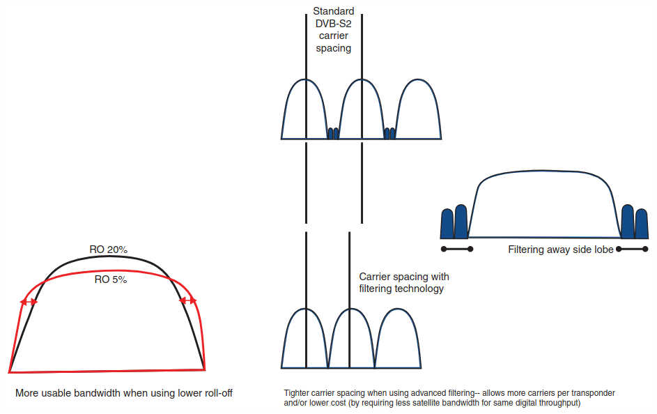
The tighter roll-off (smaller value of α) is a function of the filtering technology and could be applicable to any scheme; however, it is an intrinsic feature of DVB-S2X. Figure 14 depicts graphically the advantage of lower roll-off, in allowing less energy to spill into an adjacent band, leading to operations without excessive guard band.
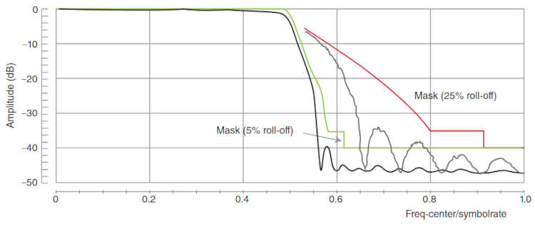
Figure 15 depicts how a tighter filtering would benefit the existing DVB-S2 standard.
To come back to DVB-S2X, the advanced filtering utilized in DVB-S2X allows elimination of side lobes next to carriers; thus the carrier spacing is reduced to only 1,05 times their symbol rates; in turn, this supports the possibility of putting carriers closer to each other, which results in BW gain (Figure 16).
DVB-S2X allows additional MODCODs compared with DVB-S2; it doubles the existing MODCOD points. More granularity means having more choices, which leads to more efficiency. Better FECs implies a lower Es/No threshold, which leads to better efficiency. Higher Modulations of 64-APSK leads to higher efficiency, up to 5 bits/Hz (see Figure 17 for the constellations).
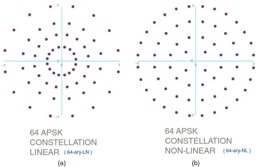
Typical modulation symbol rates are:
- 5-15, Mbaud
- 36, Mbaud
- 54, Mbaud
- 72 Mbaud.
Better implementation by the use of more sophisticated receivers, namely, a linear adaptive equalizer, or even more advanced and complex recursive decoding/demapping technologies, can significantly improve the efficiency of S2 and S2X, ranging from 5 % to 10 %. Figure 18 pulls all these concepts together to show the advantage of DVB-S2X in optimizing spectral efficiency.
DVB-S2X allows the service user to differentiate between linear operation (for a nonsaturated transponder) and nonlinear operation (for a saturated transponder). It introduces MODCODs that are less sensitive to distortion for saturated transponders by allowing the use of nonlinear MODCOD for saturated transponders and linear MODCOD for multicarrier operation. There are 87 MODCOD in total. One can select the optimal MODCOD for full transponder operation by looking at the required Es/No, the value for the optimal OBO, and the resulting nonlinear degradation.
The following 58 nonlinear MODCODs are supported:
- QPSK: 45/180, 60/180, 72/180, 80/180, 90/180, 100/180, 108/180, 114/180, 120/180, 126/180, 135/180, 144/180, 150/180, 160/180, 162/180;
- 8-PSK: 80/180, 90/180, 100/180, 108/180, 114/180, 120/180, 126/180, 135/180, 144/180, 150/180;
- 16-APSK: 80/180, 90/180, 100/180, 108/180, 114/180, 120/180, 126/180, 135/180, 144/180, 150/180, 160/180, 162/180;
- 32-APSK: 100/180, 108/180, 114/180, 120/180, 126/180, 135/180, 144/180, 150/180, 160/180, 162/180;
- 64-APSK: 90/180, 100/180, 108/180, 114/180, 120/180, 126/180, 135/180, 144/180, 150/180, 160/180, 162/180.
The following 58 linear MODCODs are supported:
- QPSK: 45/180, 60/180, 72/180, 80/180, 90/180, 100/180, 108/180, 114/180, 120/180, 126/180, 135/180, 144/180, 150/180, 160/180, 162/180;
- 8-PSK-L: 80/180, 90/180, 100/180, 108/180, 114/180, 120/180;
- 8-PSK: 126/180, 135/180, 144/180, 150/180;
- 16-APSK-L: 80/180, 90/180, 100/180, 108/180, 114/180, 120/180, 126/180, 135/180, 144/180, 150/180, 160/180, 162/180;
- 32-APSK: 100/180, 108/180, 114/180, 120/180, 126/180, 135/180, 144/180, 150/180, 160/180, 162/180;
- 64-APSK-L: 90/180, 100/180, 108/180, 114/180, 120/180, 126/180, 135/180, 144/180, 150/180, 160/180, 162/180.
DVB-S2X can be utilized in cases where one has high SNRs (which utilize the high-order modulation schemes) and low or very low SNR environments, using the low-order MODCODs. Table 3 depicts possible MODCODs and roll-off arrangements for various applications.
| Table 3. DVB-S2X Possible MODCODs and Roll-off Arrangements for Various Applications | ||
|---|---|---|
| DVB-SX NL (RO 10 %) versus DVB-S2 (RO 20 %) | Nonlinear | |
| Efficiency (%) | #modcods | |
| Mobile (-10 – -3) | 26,77 | 6 |
| Low (-3 – 5) | 11,50 | 11 |
| Broadcast (5 – 12) | 9,53 | 15 |
| Professional (12 – 24) | 17,16 | 18 |
| Full (-10 – 24) | 16,24 | 50 |
| DVB-SX L (RO 10 %) versus DVB-S2 (RO 20 %) | Linear | |
| Efficiency (%) | #modcods | |
| Mobile (-10 – -3) | 10,01 | 6 |
| Low (-3 – 5) | 6,10 | 14 |
| Broadcast (5 – 12) | 12,19 | 20 |
| Professional (12 – 24) | 29,71 | 13 |
| Full (-10 – 24) | 16,50 | 53 |
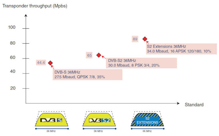
Figure 19 shows a comparison of the throughput achievable on a standard transponder using the three DVB techniques:
- DVB-S,
- DVB-S2,
- DVB-S2X.
Importantly, the DVB-S2X standard supports wideband transponders that are becoming available on satellites [especially High Throughput Satellites (HTSs)] to support high-speed data links.
The wideband implementation in DVB-S2X typically addresses satellite transponders with BWs from 72 MHz (e. g., on C-band systems) up to several hundred MHz (e. g., on Ka-band HTS systems, where a typical HTS has a significant number of ultrawide band [UWB]) transponders distributed among the beams, each with a BW of 100 MHz or more). The DVB-S2X demodulator can receive the complete wideband signal up to 72 Mbaud, resulting in a high data rate, along with an additional 20 % efficiency gain.
High-end satellite modem and modulator manufacturers (e. g., Newtec) have been conducting “record breaking demos” using production equipment. For example, in June 2012, in a two-way high-speed backbone test, Newtec achieved 506 Mbps (2 × 253 Mbps) over a 72 MHz transponder on a Eutelsat W2A.
For this test, a 32-APSK 135/180 with 5 % roll-off modulation MODCOD was used. An earlier test between Newtec and PSSI Global Services, which was conducted in preparation for the UHD demonstration, achieved 140 Mbps over a 36 MHz transponder on Galaxy 13 to a 4,6-meter antenna using to be standardized DVB-S2X technology (32-APSK 150/180, 5 % roll-off, 34,285 Mbaud).
Other press time DVB-S2X demos are as follows:
- Yahsat – 310 Mbps over a 36 MHz Ka-band transponder;
- Intelsat – 485 Mbps over a 72 MHz Ku-band transponder with BWC;
- Eutelsat – 377,5 Mbps over 72 MHz one-way in 64-APSK 162/180; and
- Newtec MDM6000 – 2 × 380 Mbps.
This technology may be useful in Ultra HD applications. For example, Intelsat and Ericsson demonstrated true UHD 4K, end-to-end video transmission via satellite in June 2013 at Turner Broadcasting in Atlanta. Intelsat’s Galaxy 13 satellite delivered a 100 Mbps, 4:2:2, 10-bit, 4K UHD signal at 60 frames per second.
Broadcast modulator, demodulator, and modem platform equipment reaching the market at press time (e. g., Newtec’s M6100 and MDM6100) was already capable of supporting DVB-S2X, DVB RF-CID, and transmodulation (DVB-S2X to DVB-S2 or to DVB-S).
The implications for satellite operators are that users may, in principle, require less transponder BW to support the same needed throughput. Or, that, considering the ever-increasing BW growth driven by evolving applications, users will simply benefit from the increased throughput thus achievable on a specified transponder BW.
Note, in conclusion, that as of press time, not all service providers (e. g., DirecTV) and terminal manufacturers have shown immediate interest (especially in consideration of any large embedded base). Also, the extension is much more complicated than DVB-S2 itself, and the high-order constellations are only for the forward link.
Other Ground-side Advances
Another recent advance is the inclusion of a Carrier Identifier (CID) in a transmitted signal.
Carrier ID
According to a recent report, 93 % of operators and users who responded to a questionnaire by the Satellite Interference Reduction Group (sIRG) suffer from interference at least once a year and 27 % suffer on a weekly basis. Embedding a CID into the carrier is a robust mechanism being developed for expeditious pinpointing of the source of satellite interference. Without automated mechanisms, manual searches are needed, which may involve expensive air-borne (e. g., helicopter-based) triangularization or other radiolocation-based technologies. Looking at the received (interfering) signal itself is the most cost-effective and reliable mechanism (when appropriate technologies are used) to identify interference issues. There is a need for standardization to support global interoperability.
Two approaches have evolved of late:
- Approach (Phase) 1: Embed Carrier ID in DVB Network Information Table (NIT) (by the World Broadcasting Unions’ International Satellite Operations Group (WBU-ISOG), as proposed in 2009); supports MPEG TS-based video carriers. It entails changes to the NIT in the original stream. It is a low robustness approach; for example, the CID is not recoverable if the main carrier is inoperative. This approach requires the insertion of CID Information in the MPEG Stream from WBU-ISOG (2011-11-09). The Encoder/Mux inserts descriptors into the NIT, and the carrier ID can be edited on the modulator. The 80 character ID includes Equipment Manufacturer; Equipment Serial Number; Telephone Number; CID; Longitude and Latitude; and User Information. In multiuplink and multihop configurations, adaptation is required. This effort has been supported by the WBU-ISOG Forum, the Global VSAT Forum (GVF), and the sIRG.
- Approach (Phase) 2: DVB Carrier ID standard (DVB-CID – 2013). With this standard, the DVB-CID signal is an overlay to original carrier; this approach is agnostic to traffic carrier or transport mechanism (TS video and IP data). It provides high robustness: it can be decoded even if the main carrier is jammed. The RF carrier ID standard was released by DVB as Bluebook A164 on February 28, 2013. It was adapted as ETSI TS 103 129 v1.1.1 in May 2013. The CID was injected by modulator into carrier with fixed source ID such as MAC address and user configurable data such as GPS coordinates, carrier name, and contact information. The WBU-ISOG Forum (May 15–16, 2013) issued a resolution in support of the ETSI TS 103 129 v1.1.1 (2013 – 05).
The DVB Carrier ID standard is the preferred method in the long term. It will enable the operators and users to rapidly identify interfering carriers and respond to Radio Frequency Interference (RFI), shortening the duration of each event.
The DVB–CID data resides under the noise floor for the Rx. The impact on overall link budget degradation of main carrier is typically less than 0,28 dB. The BW used is 224 kHz if symbol rate (SR) ≥ 512 kBaud; or 112 kHz if SR < 512 kBaud. The carrier is 220 Hz offset compared with the main signal carrier (Figure 20).
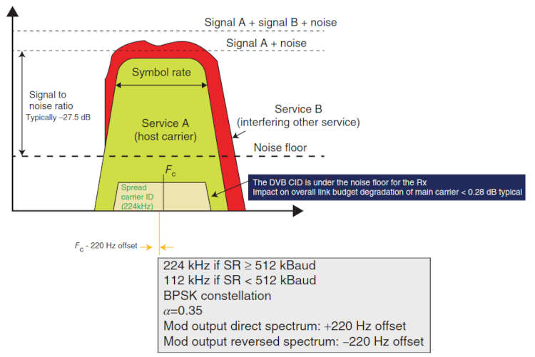
The minimum content of the Carrier ID is the DVB–CID Global Unique Identifier (GUI), fixed by the equipment manufacturer. In addition, it may contain other information that is configurable by the user, such as GPS coordinates, contact phone numbers, and so on, to simplify and speed up the process to stop the interference event. For the Carrier ID to be compatible with all carriers used in satellite today and easy to be included in all satellite modulators, the CID waveform is superimposed on the Host Data Carrier. The system uses BPSK spread spectrum modulation, differential encoding, scrambling, and a concatenated error protection strategy on the basis of repetition, cyclic redundancy check (CRC), and BCH codes.
The CID carrier is assigned a power spectrum density level well beneath the data carrier level, thus allowing for a negligible degradation of the Data Carrier performance (typically below 0,1 dB). At the same time, the adoption of Spread Spectrum technique, together with the Differentially Encoded BPSK modulation and a BCH FEC protection, allows for a very robust Carrier ID system. It should, in fact, be possible, in most practical cases, to identify the interferer without switching off the wanted signal, as particularly required by broadcast services. Manufacturers were in the process of bringing the technology to market in their modem products as of press time.
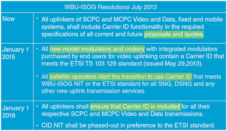
Figure 21 depicts WBU-ISOG resolutions regarding Carrier ID made in 2013.
Intelligent Inverse Multiplexing
Inverse multiplexing, the ability to provide transparently higher BW to the endpoints by “stitching together” a group of lower-speed facilities within the transport network, has been around commercially in terrestrial networks for at least 20 years, and longer than that for internal-provider-network applications. Recently, this technology has become available to satellite applications. Not only disaggregated BW on a single or multiple transponders on a satellite but also BW across multiple satellites can be “bonded” by an intelligent inverse multiplexer (I2M); in this case sophisticated timing management mechanisms (particularly buffer management and synchronization algorithms) have to be implemented in the modems (Figure 22).
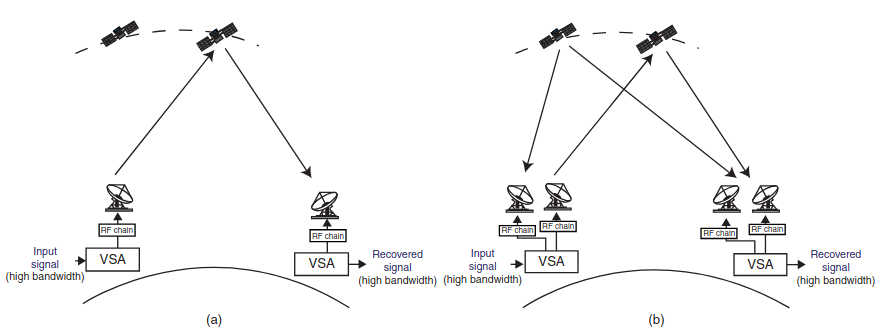
Commercial products typically combine the I2M technology with a modem capability in the same device. I2M technology may be employed in the areas of VSAT networks, cellular backhaul trunking, and possibly for Ultra HD. The challenge is to develop a modem with an acceptable price point; currently, the products are about 5–10x the cost of a normal satellite modem.
Traditionally, when information (e. g., data, voice, or video) is transported via satellite, a carrier signal is assigned a specific frequency range into which the carrier signal is placed, using FDMA principles. A satellite operator’s transponders accommodate multiple customers with each assigned a specific-sized block or BW that meets their needs. However, over the course of time and as customer requirements change, BW gaps are created, and these gaps represent unused capacity to the satellite operator. BW aggregation enables the customer to utilize these gaps as if they were one contiguous block; this is achieved by combining each block’s information-carrying capability to form a higher capacity channel. For the satellite operator this provides more opportunities to sell unused fragmented satellite capacity, and the customers get a more flexible network to improve their services (Figure 23).

There are some additional advantages to using inverse multiplexing techniques, in addition to BW aggregation: intelligent satellite BW management technology can deliver significant additional advantages, namely, interference mitigation, hitless BW adjustment, and virtualization of physical layers to incorporate fiber and satellite aggregation. Another such advantage is security (confidentiality, integrity, and availability): in the traditional approach, a customer’s content is typically encrypted and transmitted via a single carrier; an I2M allows the information to be spread across multiple carriers, each with its own and unique encryption key, making it more difficult to compromise the content by an intruder (Figure 24).
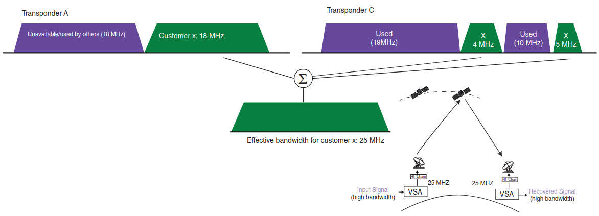
Another benefit relates to interference mitigation and antijamming: when interference occurs, it typically appears in a section of the (transponder) spectrum. In the traditional single-carrier situation, a hit by an interfering signal causes the information channel to either be rendered completely useless or be severely degraded. However, if the information is sent over multiple carriers, which have been intentionally separated in frequency using I2M technology, the impact of interference is greatly reduced; in many cases it may be completely transparent to the customer. The same methodology is applicable to the intentional jammer scenario (Figure 25).
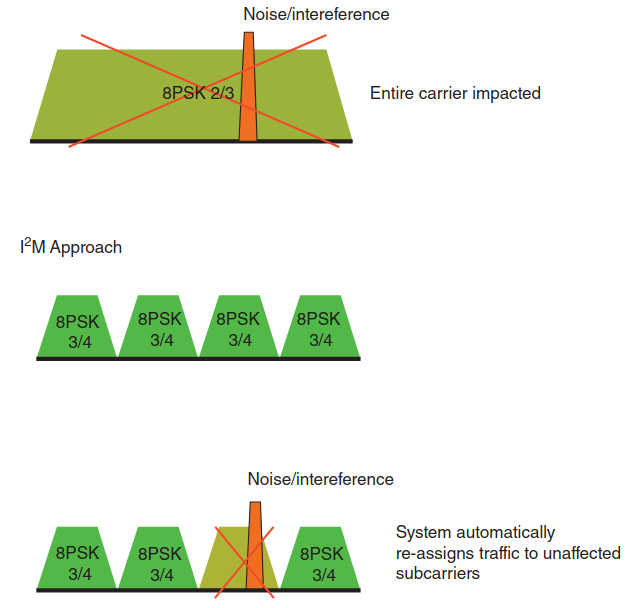
Recently (at the Satellite 2013 trade show), Alcatel-Lucent demonstrated a satellite modem platform, the Virtual Spectrum Aggregator (VSA) that supports I2M technology; the multimodem provides BW aggregation capabilities, namely, the functionality described above. The VSA expands the possibilities to how networks are designed for efficiency, flexibility, and robustness, and how satellite BW can be offered, especially in capacity-constrained situations. A throughput in the Gbps range is possible via the aggregation of multiple transponders and/or the seamless inclusion of terrestrial links for hybrid (satellite-terrestrial) networks.
As noted earlier, the concept of inverse multiplexing (also known as channel bonding) is not new. There are traditional ways of doing inverse multiplexing, such as Ethernet Link Aggregation, that rely on layer 2/3 header fields for the classification of traffic into flows that are mapped to randomly chosen physical channels. The drawback of this approach is its inability to deal with traffic comprising just a single flow – such as a video streaming session or a large file transfer – all of which maps onto a single physical link and keeps other links unused.
That same scheme is also incapable of dealing with traffic such as TSs over DVB–ASI that does not natively carry any layer 2/3 information: broadcast video requires adaptation over a layer 2/3 transport mechanism before it can be inverse multiplexed using traditional inverse multiplexing, and this approach wastes BW. The VSA technology addresses these limitations, according to the vendor, thus allowing satellite operators to utilize their transponder capacity for both video and data traffic even in the presence of fragmented spectrum. Support for up to 64-QAM constellations allows setup of high throughput links with a high degree of resiliency following the multiple levels of interference mitigation options.
For example, an IP trunk can be set up using multiple disjoint carriers such that a complete loss of one of the carriers – either because of interference or equipment failure – is hitless, from a packet delivery perspective. Another option is the rapid and automatic reconfiguration of the IP trunk in the event of a complete loss of one of the carriers. Being able to increase the spectral BW (for increased throughput) without interrupting the service is another advantage of this technology. The VSA technology is flexible; press time releases supported aggregation of up to four links with aggregate throughput of up to 1 Gbps – higher aggregate BW and number of links is possible.
Implications of H.265 Coding
HEVC is a newly developed standard. It has the same general structure as MPEG-2 and H.264/AVC, but it affords more efficient compression; namely, it can provide the same picture quality as the predecessor but with a (much) lower data rate (and storage requirement), or it can provide better picture quality than its predecessor but at the same data rate (and storage requirement). The operative feature is that video can be compressed into a smaller size or bit rate; savings ranging from 30 % to 50 % have been cited in the literature (i. e., up to 2 × better compression efficiency compared to the baseline H.264/AVC algorithm). Many demonstrations and simulations were developed in recent years, especially in 2013, and commercial-grade products are expected in the 2014–2015 timeframe, just in time for Ultra HD applications. The implications for satellite operators are that users may, in principle, require less transponder BW to support the same needed video quality or, that, considering the ever-increasing BW growth driven by evolving applications such as Ultra HD, users will either increase the video quality and retain the same transponder BW or possibly need more BW when Ultra HD services are implemented. The topic is revisited in greater detail in M2M Developments and Satellite Applications“Exploring Innovations and Applications of M2M Technology”.
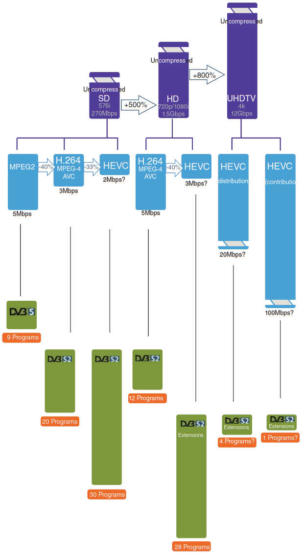
Figure 26 provides a summary of the implications of the technologies discussed (or alluded to) in this article.

- Agilent Technologies, “Digital Modulation in Communications Systems – An Introduction”, Application Note 1298, March 14, 2001, Doc. 5965-7160E, 5301 Stevens Creek Blvd, Santa Clara, CA, 95051, United States.
- A. Ambroze, M. Tomlinson and G. Wade, “Magnitude Modulation for Small Satellite Earth Terminals using QPSK and OQPSK”, Proceedings of IEEE ICC2003 conference in Alaska, USA, May 2003. IEEE, Piscataway, NJ. Faculty of Technology, University of Plymouth, Drake Circus, Plymouth PL4 8AA, United Kingdom.
- F. Amoroso, R.A. Monzingo, “Analysis Of Data Spectral Regrowth From Non-linear Amplification”, IEEE, ICPWC’97, 1997, pg 142 ff.
- C. Angelini, “Next-Gen Video Encoding: x265 Tackles HEVC/H.265”, Tom’s Hardware online magazine, July 23, 2013.
- ANS T1.523-2001, Telecom Glossary 2000, American National Standard (ANS), an outgrowth of the Federal Standard 1037 series, Glossary of Telecommunication Terms, 1996.
- B. Bross, et al., “High Efficiency Video Coding (HEVC) text specification draft 10 (for FDIS & Last Call)”, Output Document of JCT-VC, 12th Meeting: Geneva, CH, 14–23 Jan. 2013, Joint Collaborative Team on Video Coding (JCT-VC) of ITU-T SG 16 WP 3 and ISO/IEC JTC 1/SC 29/WG 11.
- D. Breynaert, M. d’Oreye de Lantremange, “Analysis of the Bandwidth Efficiency of DVB-S2 in a Typical Data Distribution Network”, Newtec, CCBN2005, Beijing, March 21–23 2005.
- J. Chen, “Extracting and Using J-models to Estimate ACPR in Direct Conversion Transmitters”, Candence White Paper, 2655 Seely Avenue, San Jose, CA 95134.
- CM701/DT7000 Reed–Solomon (DVB Version), Option Card, Com-Stream Corporation, A Spar Company, 6350 Sequence Drive, San Diego, California 92121–2724, 1998.
- DVB Carrier Identification, DVB’s Caller-ID solution to stop satellite interference, DVB Fact Sheet – August 2013.
- J. Gill, “Definition of BCH Codes”, Stanford University Lecture Notes, November 2012.
- H. Hendrix, “Viterbi Decoding Techniques for the TMS320C54x DSP Generation”, Texas Instruments, Application Report SPRA071A – January 2002. Texas Instruments.
- L. Litwin, “Error Control Coding in Digital Communications Systems”, RF Design, Jul 1, 2001.
- M. Luby, L. Vicisano, J. Gemmell, L. Rizzo, M. Handley, J. Crowcroft, “The Use of Forward Error Correction (FEC) in Reliable Multicast”, Request for Comments: 3453, December 2002.
- G. Maral, M. Bousquet, “Satellite Communications Systems: Systems, Techniques and Technology”, 2002, Wiley, New York.
- D. Marpe, H. Schwarz, and T. Wiegand, “Context-Based Adaptive Binary Arithmetic Coding in the H.264/AVC Video Compression Standard”, IEEE Transactions on Circuits and Systems for Video Technology, VOL. 13, NO. 7, JULY 2003.
- A. Morello and V. Mignone, “DVB-S2— Ready for Lift Off”, Digital Video Broadcasting, EBU TECHNICAL REVIEW – October 2004, RAI Radiotelevisione Italiana.
- Newtec Technical Materials, Newtec Cy N.V., Laarstraat 5, B-9100 Sint-Niklaas, Belgium.
- C. Placido, “Vinay Purohit, CTO Alcatel-Lucent Ventures”, Satcom Post, August 2, 2013.