Development of Natural Gas Liquefaction Cycles based on Energy and Exergy Analyses

One of the most important sections in the LNG supply chain is the energy consumption in natural gas liquefaction utilizing the energy-intensive refrigeration cycles. Therefore, selection and development of efficient refrigeration cycles to liquefy natural gas offer potential energy savings and cost benefits. The cycle selection can best be evaluated by energy and exergy analyses.

Introduction

The first law of thermodynamics is the theoretical basis of energy analysis. It is simply an energy conservation principle, asserting that energy is a thermodynamic property and that during a reaction, energy can change from one form to another but total amount of energy remains constant. An energy analysis of an energy-conversion system is essentially an accounting of the energies entering and exiting. The exiting energy can be broken down into products and wastes (for refrigeration cycle, they are typically refrigeration effect and heat and/or mechanical losses). Efficiencies often are evaluated as ratios of product energy to the energy quantities in the feed streams, and are often used to assess and compare various systems. However, energy analysis is often insufficient to evaluate system perfor-mance in that it cannot quantify the performance of a system compared to an ideal cycle (Carnot or reverse Carnot cycle). Further, energy analysis only takes into account the quantity of the thermo-dynamic losses that occur within a system, rather than the quality of the energy (potential to produce work).

Exergy analysis permits many of the shortcomings of energy analysis to be overcome. Exergy analysis is based on the second law of thermodynamics, and is useful in identifying the causes, locations, and magnitudes of process inefficiencies. Exergy (or availability) is a thermodynamic property that represents the maximum work that can be done with a given fluid stream in a reversible process Exergy is defined only in terms of enthalpy and entropy of the system that is brought to equilibrium with its surroundings in a hypothetical reversible process. The change of this property states the maximum amount of useful work that can be produced (or the minimum work that needs to be supplied) as a system undergoes a process change between the specified initial and final states.x. Thus, the exergy associated with an energy quantity is a quantitative assessment of its usefulness or quality.

As an energy-conversion system, the real liquefaction/refrigeration cycle includes various irre-versible processes. It is of great importance to analyze work losses and thermodynamic efficiency at low temperatures to avoid excessive power consumption. Therefore, the energy and exergy analyses provide a very important criterion to evaluate the thermodynamic performance of a liquefaction/refrigeration system. By analyzing the irreversibility of the system, it can be known how the actual cycle deviates from the ideal cycle. Exergy analysis is usually aimed at determining the maximum performance of the system and identifying the locations of exergy destruction and to show the direction for potential improvements.

An important object of exergy analysis for systems that consume work such as liquefaction of gases is finding the minimum work required for a certain desired result and comparing it to the actual work consumption. The ratio of these two quantities is often considered the exergy efficiency of such a liquefaction process. In recent decades, exergy analysis has been accepted as an alternative tool to traditional energy analyses for evaluation of cryogenic cycle optimization In general, cycle work consumption and/or exergy efficiency are chosen as the objective of optimization.x.

An exergy analysis of a complex system can be performed by analyzing the components of the system separately. The general principles and methodologies of exergy analysis have been published in various textbooks and are not repeated in this chapter. In this chapter, theoretical and practical aspects of energy and exergy analyses that are most relevant to refrigeration and natural gas liquefaction cycles are described. The first section reviews fundamental principles of refrigeration and liquefaction cycles. The second section summarizes the category of various refrigerants and cryogenic fluids. The third section reviews relevant theories of energy and exergy modeling and analysis. The last section provides the case analysis of some natural gas liquefaction cycles using the methods and theories introduced in the previous sections.

Refrigeration/liquefaction cycle principles

Constant-temperature refrigeration cycle

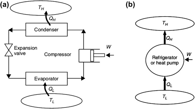
A refrigerator is a device used to transfer heat from a low- to a high-temperature medium. They are cyclic devices. Figure 1 a shows the schematic of a vapor-compression refrigeration cycle (the most common type). The working fluid (called refrigerant) absorbs heat (​\( \style{font-size:22px}{Q_L} \)​) from a low-temperature medium (at ​\( \style{font-size:22px}{T_L} \)​) in the evaporator. Power (​\( \style{font-size:22px}W \)​) is added in a compressor to compress the refrigerant to the condensing pressure. The high-temperature refrigerant cools into the liquid phase by rejecting the heat (​\( \style{font-size:22px}{Q_H} \)​) to a high-temperature medium (at ​\( \style{font-size:22px}{T_H} \)​) in the condenser. The refrigerant in the liquid phase enters the expansion valve and is expanded to give a low temperature and pressure two-phase mixture at the evaporator inlet. The cycle is demonstrated in a simplified form in Figure 1 b.

The Carnot cycle is a theoretical model that is useful for understanding a refrigeration cycle. As known from thermodynamics, the Carnot cycle is a model cycle for a heat engine where the addition of heat energy to the engine produces work. Conventionally, the Carnot refrigeration cycle is known as the reversed Carnot cycle (Figure 2). The maximum theoretical performance can be calculated, establishing criteria against which real refrigeration cycles can be compared.

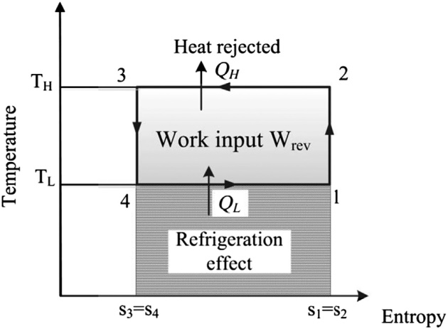
The following processes take place in the Carnot refrigeration cycle as shown on a temperature-entropy (T-s) diagram in Figure 3:

1. (​\( \style{font-size:22px}{1\rightarrow2} \)​) is the ideal compression at constant entropy, and work input is added. The temperature of the refrigerant increases.
2. (​\( \style{font-size:22px}{2\rightarrow3} \)​) is the rejection of heat to the surrounding at a temperature ​\( \style{font-size:22px}{T_H} \)​.
3. (​\( \style{font-size:22px}{3\rightarrow4} \)​) is the ideal expansion at constant entropy. The temperature of the refrigerant decreases.
4. (​\( \style{font-size:22px}{4\rightarrow1} \)​) is the absorption of heat from the heat source at a constant evaporation temperature ​\( \style{font-size:22px}{T_L} \)​.

The heat transfer between the refrigerator and the heat source/sink is assumed to occur at a zero temperature difference in all reversible refrigerators. The condensing and evaporating temperatures of the refrigerant are therefore the same as that of the ambient (​\( \style{font-size:22px}{T_H} \)​) during the heat rejection process and that of the load (​\( \style{font-size:22px}{T_L} \)​) during the heat absorption process, respectively.

The refrigeration effect ​\( \style{font-size:22px}{Q_L} \)​ is represented as shown here:

Based on the first law of thermodynamics, the theoretical work input (e.g., compressor work) for the reverse cycle (​\( \style{font-size:22px}{W_{rev}} \)​) is represented as the area within the cycle line 1-2-3-4-1, as follows:

The coefficient of performance (​\( \style{font-size:22px}{COP} \)​) of any refrigerator is defined as the ratio of heat absorbed at a low temperature to compressor work input:

This relation indicates that ​\( \style{font-size:22px}{COP} \)​ for the reverse cycle depends only on the source/sink temperatures (​\( \style{font-size:22px}{T_H} \)​ and ​\( \style{font-size:22px}{T_L} \)​), not on the thermal-physical properties of the working fluids. In order to increase the cycle ​\( \style{font-size:22px}{COP} \)​, ​\( \style{font-size:22px}{T_H} \)​ should be decreased but ​\( \style{font-size:22px}{T_L} \)​ should be increased as much as possible. Besides, variation of heat sink temperature ​\( \style{font-size:22px}{T_L} \)​ has more influence on the cycle ​\( \style{font-size:22px}{COP} \)​ than variation of heat source temperature ​\( \style{font-size:22px}{T_H} \)​. Therefore, the derivative of Equation 4 should satisfy with the following inequality equation:

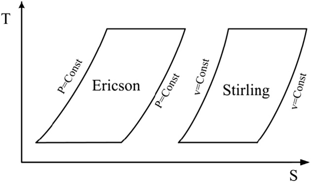
The Ericsson and Stirling cycles are principally of theoretical interest as examples of cycles that exhibit the same thermal efficiency as the reverse Carnot cycle. As shown in Figure 4, they respectively have two constant-pressure and constant-volume processes, replacing the constantentropy processes in the reverse Carnot cycle.

Irreversible refrigeration cycle with finite heat transfer temperature differences

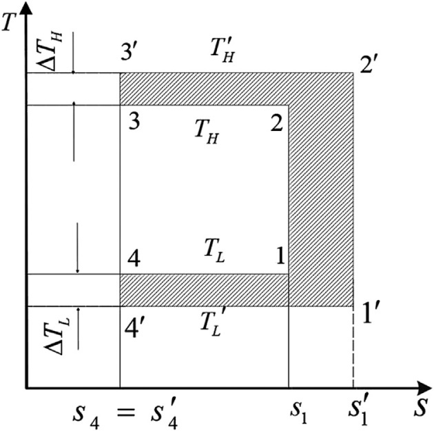
The analysis in Section 4.2.1 assumes zero temperature difference between the working fluid (refrig-erant) and ambient/load at heat rejection and absorption processes, respectively. However, such zero heat transfer temperature difference requires an infinitely large area of the heat exchanger, which is impossible for practical applications. In reality, in the heat rejection process the temperature of the working fluid (​\( \style{font-size:22px}{T_H’} \)​) is higher than the ambient temperature (​\( \style{font-size:22px}{T_H} \)​ ), and in the heat absorption process the working fluid temperature (​\( \style{font-size:22px}{T_L’} \)​) is lower than the load temperature (​\( \style{font-size:22px}{T_L} \)​).When ​\( \style{font-size:22px}{T_H} \)​ and ​\( \style{font-size:22px}{T_L} \)​ are fixed, the reverse refrigeration cycle with finite heat transfer temperature difference is denoted as ​\( \style{font-size:22px}{1′-2′-3′-4′-1′} \)​ in Figure 5.

Since heat transfer through a finite temperature difference is an irreversible process, this cycle with two constant-entropy and two heat transfer processes is a reverse Carnot cycle with external irreversibility. ​\( \style{font-size:22px}{Q_H’} \)​ and ​\( \style{font-size:22px}{Q_L’} \)​ represent the heat rejection and the cooling capacity in the irreversible cycle, respectively. Thus, according to the first law of thermodynamics:

The internal reversible cycle:

The external irreversible cycle:

Due to finite heat transfer temperature differences ​\( \style{font-size:22px}{\Delta T_H-T_H’-T_H} \)​ and ​\( \style{font-size:22px}{\Delta T_L-T_L-T_L’} \)​, the range of the cycle temperature is increased; that is, ​\( \style{font-size:22px}{(T_H’-T_L’)>(T_HT_L)} \)​ and ​\( \style{font-size:22px}{T_L'<T_L} \)​. Compared with the reversible Carnot cycle 1-2-3-4-1, the coefficient of performance for the cycle with heat transfer temperature difference is lower than that with zero temperature difference; that is, ​\( \style{font-size:22px}{COP_{irrev}<COP_{rev}} \)​. If two cycles produce the same refrigeration capacity ​\( \style{font-size:22px}{Q_L=Q_L’} \)​, the additional work required by the irreversible cycle (​\( \style{font-size:22px}{1′-2′-3′-4′-1′} \)​) can be expressed as

This indicates that the value of the additional work input (​\( \style{font-size:22px}{\Delta W} \)​) is equal to the difference of heat rejection to the ambient in the irreversible cycle and in the reversible cycle. In Figure 5, ​\( \style{font-size:22px}{\Delta W} \)​ can also be represented as the shadow area difference within two cycle lines. Entropy generation in this irreversible cycle is due to heat transfer at ​\( \style{font-size:22px}{\Delta T_H>0} \)​ and Δ​\( \style{font-size:22px}{T_L>0} \)​. Thus, the total entropy generation can be expressed as

Since in the reversible cycle the entropy generation ​\( \style{font-size:22px}{\Delta S_{rev}=-\frac{Q_H}{T_H}+\frac{Q_L}{T_L}=0} \)​, Equation 6 can be simplified to

Using the relationships in the T-s diagram, the following equation can be derived:

Substituting Equations 5 and 9 into Equation 8, the entropy generation can be expressed as

Thus,

Equation 11 demonstrates that to obtain the same amount of cooling capacity, additional work input for the irreversible refrigeration cycle is equal to the ambient temperature (​\( \style{font-size:22px}{T_H} \)​) multiplied by the entropy generation in the system (​\( \style{font-size:22px}{DS_{irrev}} \)​).

Refrigeration cycle between two varying temperatures

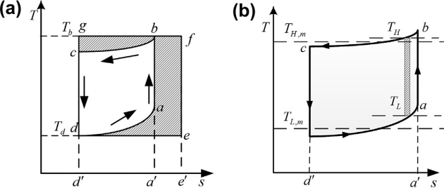
In a real refrigeration cycle, the temperatures of the low temperature medium (heat source) and the high temperature medium (heat sink) are usually varying. In this case, we can assume that the heat source is cooled down from ​\( \style{font-size:22px}{T_a} \)​ to ​\( \style{font-size:22px}{T_d} \)​ and the heat sink is heated up from ​\( \style{font-size:22px}{T_c} \)​ to ​\( \style{font-size:22px}{T_b} \)​, as shown in Figure 6 a. Line ​\( \style{font-size:22px}{a-d} \)​ and ​\( \style{font-size:22px}{c-b} \)​ represent thermodynamic processes of the heat source and the heat sink, respectively; area within the line ​\( \style{font-size:22px}{a’-a-d-d’\;-a’} \)​ represents the cooling capacity ​\( \style{font-size:22px}{Q_L} \)​. Under conditions just given, in order to consume the minimum input work, cycle ​\( \style{font-size:22px}{a-b-c-d-a} \)​ is assumed to be a reversible refrigeration cycle. Heat transfer temperature differences between the refrigerant and the heat source/sink are assumed to be infinitely small. Therefore, thermal state lines of the refrigerant ​\( \style{font-size:22px}{d-a} \)​ and​\( \style{font-size:22px}{\;b-c} \)​ represent the heat absorption process from the low temperature medium (heat source) and the heat rejection process to the high temperature medium (heat sink), respectively; arrows indicate the direction of the reversible refrigeration cycle.

Process ​\( \style{font-size:22px}{a-b} \)​ and ​\( \style{font-size:22px}{c-d} \)​ are the reversible adiabatic compression and expansion. It can be seen that the cycle ​\( \style{font-size:22px}{a-b-c-d-a} \)​ is a reversible cycle without work loss due to the entropy generation. Therefore, the work input for this cycle (​\( \style{font-size:22px}{W_0} \)​) is minimum, and ​\( \style{font-size:22px}{COP=\frac{Q_L}{W_0}.} \)​

For the reversible Carnot cycle with varying temperatures, its ​\( \style{font-size:22px}{COP} \)​ can be presented based on average equivalent temperatures. As shown in Figure 6 b, we can use a series of adiabatic lines to divide the Carnot cycle ​\( \style{font-size:22px}{a-b-c-d-a} \)​ into infinite numbers of element Carnot cycles. For each element cycle, heat source temperature ​\( \style{font-size:22px}{T_{H,\;i}} \)​ and heat sink temperature ​\( \style{font-size:22px}{T_{L,\;i}} \)​ can be assumed to be constant. Thus, its ​\( \style{font-size:22px}{COP_i} \)​ is

For the entire Carnot cycle, ​\( \style{font-size:22px}{COP} \)​ can be expressed as

The heat exchange can be expressed as

 where ​\( \style{font-size:22px}{T_{L,m}} \)​ is defined as the average equivalent temperature of working fluid absorbing heat from the heat source, which indicates that the amount of heat absorption at the constant ​\( \style{font-size:22px}{T_{L,m}} \)​ is equal to that at varied temperatures in process ​\( \style{font-size:22px}{d-a} \)​. Similarly, ​\( \style{font-size:22px}{T_{H,m}} \)​ is the average equivalent heat rejection temperature.

Substituting Equations 14 a and 14 b into Equation 13, ​\( \style{font-size:22px}{COP} \)​ for the reversible Carnot cycle at varied temperatures can be written as

Liquefaction of gases

Liquefaction of gases is always accomplished by refrigerating the gas to some temperature below its critical temperature so that liquid can be formed at some suitable pressure below the critical pressure. Thus, gas liquefaction is a special case of gas refrigeration and cannot be separated from it. In both cases, the gas is first compressed to an elevated pressure in an ambient temperature compressor. This high pressure gas is passed through a countercurrent recuperative heat exchanger to a throttling valve or expansion engine, as shown in Figure 7. Before expanding to the lower pressure, cooling may take place, and some liquid is formed. The cool, low pressure gas is returned to the compressor inlet to repeat the cycle. The purpose of the countercurrent heat exchanger is to warm the low-pressure gas prior to recompression and simultaneously to cool the high-pressure gas to the lowest temperature possible prior to expansion. Both refrigerators and liquefiers operate on this basic principle.

There is nonetheless an important distinction between refrigerators and liquefiers. In a continuous refrigeration process, there is no accumulation of refrigerant in any part of the system. This contrasts with a gas liquefying system, where liquid accumulates and is withdrawn. Thus, in a liquefying system, the total mass of the gas that is warmed in the counter-current heat exchanger is less than that of the gas to be cooled by the amount liquefied, creating an imbalance of flow in the heat exchanger. In a refrigerator, the warm and cool gas flows are equal in the heat exchanger. This results in what is usually referred to as a “balanced flow condition” in a refrigerator heat exchanger. The thermodynamic principles of refrigeration and liquefaction are identical. However, the analysis and design of the two systems are quite different because of the condition of balanced flow in the refrigerator and unbalanced flow in liquefier systems.

The prerequisite refrigeration for gas liquefaction is accomplished in a thermodynamic process when the process gas absorbs heat at temperatures below that of the environment. As mentioned, a process for producing refrigeration at liquefied gas temperatures always involves some equipment at ambient temperature in which the gas is compressed and heat is rejected to a coolant. During the ambient temperature compression and cooling process, the enthalpy and entropy, but not usually the temperature of the gas, are decreased.

The reduction in temperature of the gas usually is accomplished by recuperative heat exchange between the cooling and warming gas streams and further by an expansion of the high-pressure stream. One method of producing low temperatures is the isenthalpic expansion through a throttling device. The effect has come to be known as the Joule-Thomson effect, and the Joule-Thomson coefficient (​\( \style{font-size:22px}{\mu_{J-T}} \)​) of a gas is defined as follows:

The Joule-Thomson coefficient is a property of each specific gas, a function of temperature and pressure, and may be positive, negative, or zero.

Another method of reducing gas temperatures is the adiabatic expansion of the gas through a work-producing device such as an expansion engine. In the ideal case, the expansion would be reversible and adiabatic and therefore isentropic. In this case, the isentropic expansion coefficient ​\( \style{font-size:22px}{\mu_S} \)​ is defined as follows, which expresses the temperature change due to a pressure change at constant entropy.

The isentropic expansion process removes energy from the gas in the form of external work, so this method of low-temperature production is sometimes called the external work method. Expansion through an expansion valve does not remove any energy from the gas but moves the molecules farther apart under the influence of intermolecular forces, so this method is called the internal work method.

Ideal Linde-Hampson liquefiers

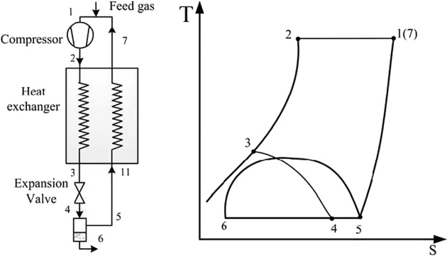
Figure 8 shows an ideal Linde-Hampson liquefier, originally invented by Carl von Linde and William Hampson independently in 1895 to liquefy air, and the corresponding temperature-entropy (​\( \style{font-size:22px}{T-s} \)​) diagram. In an ideal liquefaction system, the gas to be liquefied is compressed in a process of multistage adiabatic compression and multistage isobaric cooling. Therefore, this process is regarded as isothermal compression at ambient temperature (1-2). The high-pressure gas is cooled in the heat exchanger (2-3) and then expanded isenthalpic in a throttling device (3-4). The liquid (6) and gaseous phases (5) are separated in the phase separator, and the unliquefied gas is used to cool the high-pressure warm stream in the heat exchanger. The temperature of the low-pressure return gas at the exit of the heat exchanger depends on the effectiveness of the heat exchanger used. In the case of an ideal heat exchanger with a heat exchanger effectiveness of 100 %, ​\( \style{font-size:22px}{T_7\;=\;T_1} \)​.

In order to quantify the fraction of the gas that gets liquefied (the liquid yield (​\( \style{font-size:22px}y \)​) in an ideal Linde-Hampson process), ​\( \style{font-size:22px}y \)​ kg gas is liquefied from 1 kg feed gas after compression, cooling, and expansion. Taking a control volume that includes the heat exchanger, the expansion valve, and the phase separator, the energy conservation gives

Therefore, the liquid yield ​\( \style{font-size:22px}y \)​ can be expressed as

where ​\( \style{font-size:22px}{h_1,\;h_2} \)​, and ​\( \style{font-size:22px}{h_6} \)​ represent enthalpy at corresponding state points of 1, 2, and 6.

Ideal liquefiers with expanders

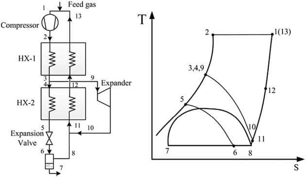
Figure 9 shows an ideal expander liquefier and the corresponding temperature-entropy diagram. A large part of the high pressure gas is diverted to an expander and undergoes a large temperature drop. This cold gas is used to cool and condense the high-pressure gas in the second heat exchanger (HX-2). The refrigeration obtained in the expander also helps in precooling the high-pressure gas in the first heat exchanger (HX-1) before it enters the expander and the second heat exchanger (HX-2).

Similarly, the expression for liquid yield (​\( \style{font-size:22px}y \)​) in this liquefier is obtained by an energy balance over a control volume that excludes the compressor as follows:

where ​\( \style{font-size:22px}{h_1,\;h_2,\;h_7,\;h_9} \)​, and ​\( \style{font-size:22px}{h_{10}} \)​ represent enthalpy at corresponding state points of 1, 2, 7, 9, and 10; m is the fraction of gas passing through the expander

Refrigerant selections

Applications requiring refrigeration are extremely diverse and broad-based. They span a broad range of temperatures ranging from near absolute temperature (liquid helium) of 4 K to near ambient temperature (human comfort) of 300 K. Apart from the refrigeration temperature, the refrigeration capacity requirement also plays a significant role in influencing the refrigeration method and refrigerants that can be employed. Practices in the industry also show that for any given application, defined by its refrigeration temperature and capacity requirements, a number of different refrigeration methods and corresponding refrigerants have been implemented. In general, refrigerants are classified into two categories. The first group includes refrigerants working at nearambient temperatures. They are used in refrigerators operating as a closed loop. There is no accumulation or withdrawal of product in a refrigerator. Typical refrigerants are inorganic compounds, halocarbon compounds, and hydrocarbons. The common feature of this type of refrigerants is that they have relatively high critical temperatures and can be liquefied near ambient or medium cold temperatures. The other type is called cryogenic fluidsdcryogenic gases including methane, air, oxygen, nitrogen, and so on. They have very low boiling temperatures, usually below 120 K. Cryogenic gases are used in open liquefiers where liquid products are removed and equivalent make-up stream must be added.

Basic requirements on refrigerants

The basic requirements on the common refrigerants used for room or low temperature refrigeration are the following:

1. Critical temperatures are not too low such that refrigerants can be liquefied at ambient or medium low temperatures;
2. It should have appropriate saturation pressures at the range of the working temperatures of the refrigerator. In general, the evaporating pressure is preferred close to or higher than atmosphere pressure, preventing the air infiltrating into the low pressure components; meanwhile, the condensing pressure should not be too high, otherwise it may increase the compressor work;
3. The volumetric refrigerating capacity is high, which will reduce the size of the compressor and refrigerant flow rate;
4. Viscosity and density are small, and therefore pressure drops in the system will be low;
5. Refrigerants should have high thermal conductivity, which can increase the effectiveness of the evaporator and condenser and decrease the heat exchanger area;
6. With respect to chemical characteristics, the nontoxicity, suitable material of construction, and compatibility with lubricant are preferred.

Since the cryogenic fluids are mainly used for cryogenic applications at a working temperature below 120 K, in order to reach such extremely low working temperatures the working fluids should have a very low normal boiling temperature (below 120 K) and triple point. Any fluids with such characteristics potentially could be used as cryogenic refrigerants.

Type of refrigerants for refrigeration and liquefaction

The typical refrigerants used for refrigeration and liquefaction cycles are categorized, based on their own chemical compositions, as the following:

• Halocarbon compounds. The halocarbon compounds group includes refrigerants that contain one or more of the three halogens chlorine, fluorine, and bromine;
• Inorganic compounds. Many of the early refrigerants were inorganic compounds and some have maintained their prominence to this day, such as ammonia and carbon dioxide;
• Hydrocarbons. Many hydrocarbons are suitable as refrigerants, especially for service in the petroleum and petrochemical industry;
• Cryogenic gases. Many gases and their mixtures are used as cryogenic fluids such as nitrogen, oxygen, air, methane, helium, etc.

Type of refrigerant mixtures

Refrigerant mixtures can be broadly classified into two groups based on the temperature change during the phase change process (evaporation and condensation): (1) zeotropic mixtures and (2) azeotropic mixtures. A mixture of chemicals is zeotropic if the compositions of the vapor and the liquid phases at the vapor-liquid equilibrium state are never the same. Dew point and bubble point curves do not touch each other over the entire composition range with the exception of the pure components. An azeotropic mixture of two substances is one that cannot be separated into its components by distillation. An azeotrope evaporates and condensates as a single substance with properties that are different from those of either constituent. Typical advantages of using zeotropic mixtures for refrigeration include (1) reducing compression ratio; (2) increasing the capacity of the refrigerator; (3) reaching nonconstant temperature refrigerating (refrigerant temperature decreases at the condensation and increases at the evaporation), consequently reducing the compressor work and increasing ​\( \style{font-size:22px}{COP} \)​. With respect to azeotropic, its benefit is that at the same operating conditions, evaporating temperature is lowered compared to using either constituent. Thus, the refrigerating capacity will be increased and compressor discharge temperature will be reduced.

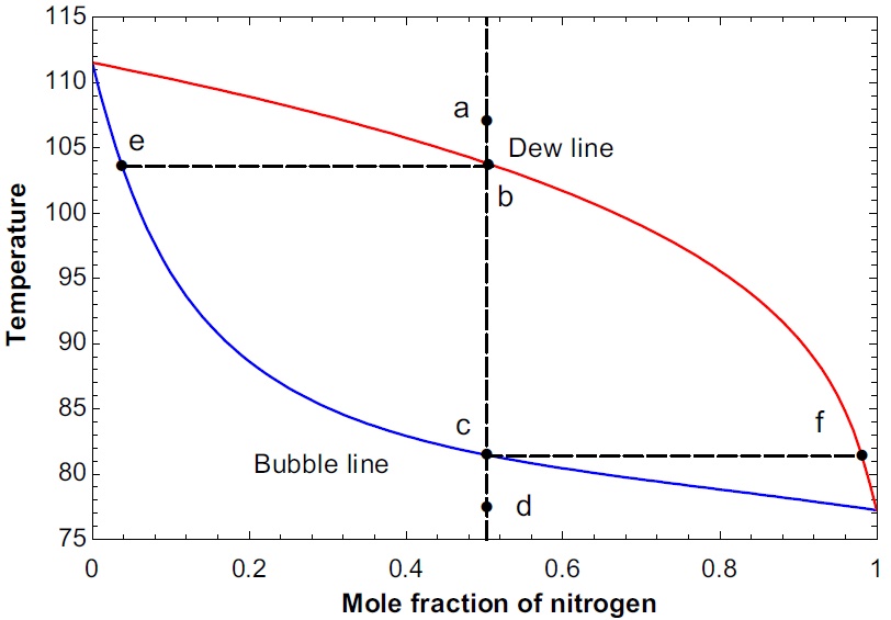
Figure 10 shows the relationship between the dew and bubble point temperatures of a typical zeotropic mixture of nitrogen and methane at a pressure of 0.1 MPa. Consider four different states, a (107.5 K), b (103.87 K), c (81.49 K), and d (77.5 K) at a nitrogen mole fraction of 0.5. The mixture is in a superheated vapor state at a, saturated vapor state at b, saturated liquid state at c, and subcooled liquid state at d. The temperature of the mixture at saturated vapor state b and at saturated liquid state c is called the dew and bubble point temperature, respectively. The line passing through the dew points is called the dew line, and that through the bubble points is called the bubble line. The equilibrium composition of vapor and liquid will be different in the two-phase region. For example, the mole fraction of vapor in equilibrium with liquid at state c will be greater than 0.5 (state f), whereas the mole fraction of liquid in equilibrium with vapor at state b would be less than 0.5 (state e).

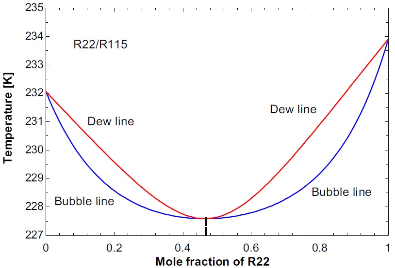
Figure 11 shows the typical variation of the dew and bubble point temperature of an azeotropic mixture of refrigerants R22 (​\( \style{font-size:22px}{CHClF_2} \)​) and R115 (​\( \style{font-size:22px}{CClF_2CF_3} \)​). The temperature glide becomes zero when the mole fraction of R22 in the mixture is 0.488. The mole fraction of the vapor and liquid phases is also the same at this mole fraction. Azeotropic mixtures are widely used for constant-temperature refrigeration. However, they are not suitable for the process described in this monograph (except as a precooling refrigerant in some cases). 

Choice of refrigerant mixture

The energy and exergy efficiency of any mixed refrigerant cycle (MRC) depends on the mixture’s constituents and their concentration. The exergy efficiency of MRC refrigerators will be high when a second liquid phase occurs in the evaporator. Liquid-liquid immiscibility is observed at low temperatures in multicomponent mixtures of nitrogen-hydrocarbon, fluorocarbon-hydrocarbon, fluorocarbon-hydrochlorofluorocarbon and fluorocarbon-hydrofluorocarbon refrigerants. This immis- cibility can be exploited to obtain a near-constant temperature evaporation with binary or multicom-ponent mixtures. The method for determining the most basic components of a nitrogen-hydrocarbon mixture was first given by Alfeev et al. (1973) in their patent. These principles later were extended to other fluid mixtures by. The proposed guidelines for choosing the components of a mixture are as follows:

1. Choose a first fluid whose boiling point temperature at 1.5 bar is less than the desired refrigerating temperature. For example, nitrogen can be used for temperatures between 80 K and 105 K, tetrafluoromethane (Refrigerant R14) between 150 K and 180 K;
2. Choose a second fluid whose boiling point is about 30 to 60 K above that of the basic fluid and that does not exhibit liquid-liquid immiscibility at low temperature with the primary fluid. For example, we can choose methane with argon and nitrogen, trifluoromethane (R23) with tetrafluoromethane (R14), etc;
3. Choose a third fluid that exhibits a liquid-liquid immiscibility at low temperature with the first fluid and whose boiling point is at least 30 K above that of the second fluid, for instance ethane, ethylene, etc., which exhibit liquid-liquid immiscibility at low temperatures with nitrogen. Ethylene also exhibits liquid-liquid immiscibility at low temperatures with argon. Propane, butanes, and chlorodifluoromethne (R22) exhibit liquid-liquid immiscibility with R14;
4. Choose a fourth and an optional fifth fluid that exhibit liquid-liquid immiscibility at low temperatures with the first fluid.

Fundamentals of energy and exergy analysis

This section introduces the thermodynamic fundamentals for energy and exergy analysis of typical components and overall cryogenic cycles.

First law and second law of thermodynamics

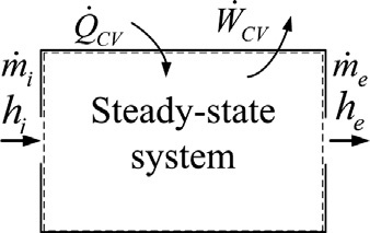
The first law of thermodynamics can be defined as the law of conservation of energy, and it states that energy can be neither created nor destroyed. It can be expressed for a general system since the net change in the total energy of a system during a process is equal to the difference between the total energy entering and leaving the system. Let us consider a control volume (CV) involving a steady-flow process. Mass is entering and leaving the system and there are heat and work interactions with the surroundings as shown in Figure 12.

During a steady-flow process, the total energy content of the control volume remains constant, and thus the total energy change of the system is zero. If the change in kinetic and potential energies are ignored, then the first law of thermodynamics can be expressed as

where i denotes inlets and e denotes exits, ​\( \style{font-size:22px}{{\dot Q}_{CV}} \)​ and ​\( \style{font-size:22px}{{\dot W}_{CV}} \)​ denote rate of energy transfer to the control volume as heat and rate of work done by the control volume, ​\( \style{font-size:22px}{\dot m} \)​ and h represent fluid mass flow rate across the boundary of the control volume and the corresponding specific enthalpy associated with the fluid flow.

However, the energy conservation idea alone is inadequate for depicting some important aspects of resource utilization. In principle, work can be developed as the systems are allowed to come into equi-librium. When one of the two systems is a suitably idealized system referred to as an exergy reference environment or an environment, and the other is some system of interest, exergy is the maximum theo-retical work obtainable as they interact to equilibrium. When mass flow is across the boundary of a control volume, there is an exergy transfer accompanying mass flow. Additionally, there is an exergy transfer accompanying flow work. The specific flow exergy accounts for both of these, and is given by

where h and s denote specific enthalpy and specific entropy, respectively; ​\( \style{font-size:22px}{\frac{V^2}2} \)​ and ​\( \style{font-size:22px}{gz} \)​ represent the specific kinetic and potential energy, respectively; ​\( \style{font-size:22px}{T_0} \)​ represents the temperature at the environment; and\( \style{font-size:22px}{h_0} \) and ​\( \style{font-size:22px}{s_0} \)​ represent the respective values of these properties when evaluated at the environment. Similarly, the exergy rate balance for a control volume in steady-state flow can be expressed as

Equation 23 a, the term ​\( \style{font-size:22px}{{\dot Q}_j} \)​ represents the time rate of heat transfer at the location on the boundary where the instantaneous temperature is ​\( \style{font-size:22px}{T_j} \)​. The accompanying exergy transfer rate is given by ​\( \style{font-size:22px}{\left(1-T_0/T_j\right){\dot Q}_j} \)​. The term ​\( \style{font-size:22px}{{\dot W}_{CV}} \)​ represents the time rate of energy transfer rate by work. The terms ​\( \style{font-size:22px}{{\dot m}_ie_{fi}} \)​ and ​\( \style{font-size:22px}{{\dot m}_ee_{fe}} \)​ account for the time rate of exergy transfer accompanying mass flow and flow work at inlet i and exit e, respectively. Finally, the term ​\( \style{font-size:22px}{{\dot E}_d} \)​ accounts for the time rate of exergy destruction due to irreversibilities within the control volume. This equation indicates that the rate at which exergy is transferred into the control volume must exceed the rate at which exergy is transferred out, the dif-ference being the rate at which exergy is destroyed within the control volume due to irreversibilities. The exergy loss ​\( \style{font-size:22px}{\Delta\dot E\left(={\dot E}_d\right)} \)​ can be expressed as:

Exergy analysis of different components of a cryogenic liquefaction system

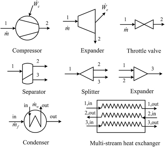
Typical components in a cryogenic liquefaction system include multistream heat exchangers, compressors, condensers, or aftercoolers exchanging heat with ambient or water, mixers, and expansion devices, as shown in Figure 13.

Ignoring the kinetic and potential energy of the working fluid, the flow exergy e in a steady state flow can be expressed as

where ​\( h \)​ and ​\( \style{font-size:22px}s \)​ represent the specific enthalpy and entropy, respectively; ​\( \style{font-size:22px}{h_0} \)​ and ​\( \style{font-size:22px}{s_0} \)​ represent the respective values of these properties when evaluated at the environment; and\( \style{font-size:22px}{T_0} \) is the environment temperature.

Compressor

According to Equation 23 b, the exergy loss in a compressor can be written as

where ​\( \style{font-size:22px}{e_1} \)​ and ​\( \style{font-size:22px}{e_2} \)​ are the specific exergy before and after the compression; ​\( \style{font-size:22px}{\dot m} \)​ is the working fluid mass flow rate; ​\( \style{font-size:22px}{{\dot W}_c} \)​ is the compressor work, and ​\( \style{font-size:22px}{-{\dot W}_c=\frac1{\eta_c}\left(h_2-h_1\right)\dot m} \)​. The exergy loss can be expressed as

In Equation 26, hc denotes the compressor efficiency.

Expander and throttle valve

The exergy loss in a throttle valve can be written as

where ​\( \style{font-size:22px}{e_1} \)​ and ​\( \style{font-size:22px}{e_2} \)​ are the specific exergy before and after the throttle process. Because of isenthalpic throttling, ​\( \style{font-size:22px}{h_1\;=\;h_2} \)​, thus the exergy loss can be expressed as

For an expander, the exergy loss based on Equation 23 b is

where​ \( \style{font-size:22px}{e_1} \)​ and ​\( \style{font-size:22px}{e_2} \)​ are the specific exergy before and after the expansion; and ​\( \style{font-size:22px}{{\dot W}_e} \)​ is the output work from the expander, and — ​\( \style{font-size:22px}{{\dot W}_e=\dot m\eta_e\left(h_2-h_1\right)} \)​. Thus, the exergy loss in an expander can be expressed as

In Equation 30, hex denotes the expander efficiency.

Stream mixer

The exergy loss in a mixer can be written as

where ​\( \style{font-size:22px}{e_1} \)​ and ​\( \style{font-size:22px}{e_2} \)​ are the specific exergy of two steams before the mixer; e₃ is the specific exergy of mixed stream. Due to energy and mass conservations, ​\( \style{font-size:22px}{{\dot m}_3h_3={\dot m}_1h_1+{\dot m}_2h_2} \)​ and ​\( \style{font-size:22px}{{\dot m}_3={\dot m}_1+{\dot m}_2} \)​, the exergy loss can be expressed as

Phase separator or stream splitter

The exergy loss in a phase separator or stream splitter can be written as

where ei, ​\( \style{font-size:22px}{e_2} \)​, and ​\( \style{font-size:22px}{e_3} \)​ are the specific exergy of main stream before the separator or splitter and two afterward streams. Similarly, the exergy loss can be expressed as

Multistream heat exchanger

The exergy loss in a multistream heat exchanger can be written as

Based on the energy conservation equation ​\( \style{font-size:22px}{\sum_i{\dot m}_{i,in}h_{i,in}=\sum_i{\dot m}_{i,out}h_{i,out}} \)​, the exergy loss can be expressed as

Water condenser or aftercooler

The exergy loss can be written as

Substituting the energy conservation equation, the exergy loss can be expressed as

In Equation 38, ​\( \style{font-size:22px}{s_{f,in}} \)​ and ​\( \style{font-size:22px}{s_{f,out}} \)​ are the specific entropy of working fluid at the inlet and outlet of the heat exchanger; ​\( \style{font-size:22px}{c_{p,w}} \)​ is the water specific heat (assumed to be constant); and ​\( \style{font-size:22px}{T_{w,in}} \)​ and ​\( \style{font-size:22px}{T_{w,out}} \)​ are water inlet and outlet temperatures, respectively.

Overall energy and exergy efficiency of a cryogenic liquefaction system

The exergy efficiency is introduced and used to assess the effectiveness of energy resource utilization in a thermal system. The exergy efficiency of any refrigeration or cryogenic liquefaction system is defined as follows:

or

For the processes or equipment (control volume) where there is no work transfer involved, the concept of exergy efficiency can also be determined. Instead, the actual power supplied is replaced by exergy expenditure as follows:

or

where ​\( \style{font-size:22px}{{\dot Q}_i} \)​ and ​\( \style{font-size:22px}{T_i} \)​ denote the obtained refrigerating effect and the corresponding refrigerating tem-perature. ​\( \style{font-size:22px}{T_0} \)​ denotes the temperature at the environment.

The exergy expenditure depends on the type of system or process. When a system receives heat and produces work as in a heat engine, the exergy expenditure of the system is ​\( \style{font-size:22px}{{\dot Q}_i(1-T_0=T_i)} \)​. When a system receives work and absorbs heat as in a refrigerator, the exergy expenditure of the system is ​\( \style{font-size:22px}{\dot W} \)​.

Energy and exergy analysis of an ideal Linde-Hampson liquefaction cycle

A methodology for the first-and second-law-based performance analyses of the simple ideal Linde- Hampson cycle was reported by Kanoglu et al. (2008), and they investigated the effects of gas inlet and liquefaction temperatures on various cycle performance parameters. The ideal Linde-Hampson cycle and its temperature-entropy diagram are shown in Figure 8. Makeup gas is mixed with the uncondensed portion of the gas from the previous cycle, and the mixture at state 1 is compressed by an isothermal compressor to state 2. The temperature is kept constant by rejecting compression heat to a coolant. The high-pressure gas is further cooled in a regenerative counterflow heat exchanger by the uncondensed portion of gas from the previous cycle to state 3, and throttled to state 4, which is a saturated liquid-vapor mixture state. The liquid (state 6) is collected as the desired product, and the vapor (state 5) is routed through the heat exchanger to cool the high-pressure gas approaching the throttling valve. Finally, the gas is mixed with fresh makeup gas, and the cycle is repeated.

The refrigeration effect for this cycle may be defined as the heat removed from the makeup gas in order to turn it into a liquid at state 6. The fraction of liquefied gas (i.e., liquid yield) can be written as

where hf is the specific enthalpy of saturated liquid that is withdrawn. From an energy balance on the cycle, the refrigeration effect per unit mass of the gas in the cycle may be expressed as

An energy balance on the heat exchanger gives

where x is the quality of the mixture at state 4. Then the fraction of the gas that is liquefied may also be related as

\[ \style{font-size:22px}{y=1-x\;\;\;\;\;\;\;\;\;\;Equation\;46} \]

An energy balance on the compressor gives the work of compression per unit mass of the gas in the cycle as

\[ \style{font-size:22px}{w_{actual}=h_2-h_1-T_1\left(s_2-s_1\right)\;\;\;\;\;\;\;\;\;\;Equation\;47} \]

The coefficient of performance (​\( \style{font-size:22px}{COP} \)​) of this ideal cycle is then given by

\[ \style{font-size:22px}{COP=\frac{q_l}{w_{actual}}=\frac{h_1-h_2}{h_2-h_1-T_1\left(s_2-s_1\right)}\;\;\;\;\;\;\;\;\;\;Equation\;48} \]

Engineers usually are interested in comparing the actual work used to obtain a unit mass of liquefied gas and the minimum work requirement to obtain the same output. Such a comparison may be performed using the second law. For instance, the minimum work input requirement (reversible work) and the actual work for a given set of processes may be related to each other by

\[ \style{font-size:22px}{w_{actual}=w_{rev}+T_0s_{gen}=w_{rev}+ex_{dest}\;\;\;\;\;\;\;\;\;\;Equation\;49} \]

where ​\( \style{font-size:22px}{T_0} \)​ is the environment temperature; ​\( \style{font-size:22px}{s_{gen}} \)​ is the specific total entropy generation; and ​\( \style{font-size:22px}{ex_{dest}} \)​ is the specific total exergy destruction during the processes. The reversible work for the simple Linde- Hampson cycle may be expressed by the stream exergy difference of states 1 and 6 as

\[ \style{font-size:22px}{w_{rev}=y\left(ex_6-ex_1\right)=y\left(h_6-h_1-T_0\left(s_6-s_1\right)\right)\;\;\;\;\;\;\;\;\;\;Equation\;50} \]

where state 1 has the properties of the makeup gas, which is essentially at the environment. This expression gives the minimum work requirement for a unit mass of the gas. The exergy efficiency can be defined as the reversible work input divided by the actual work input:

\[ \style{font-size:22px}{\eta_{ex}=\frac{w_{rev}}{w_{actual}}=\frac{y\left(h_6-h_1-T_0\left(s_6-s_1\right)\right)}{h_2-h_1-T_1\left(s_2-s_1\right)}\;\;\;\;\;\;\;\;\;\;Equation\;51} \]

Here we present a numerical example for the ideal Linde-Hampson cycle. Major assumptions are (1) a reversible and isothermal compressor; (2) an ideal heat exchanger (effectiveness = 1 and no pressure drop); (3) an ideal phase separator (no pressure drop, complete separation of phases); (4) the isenthalpic expansion process in the expansion valve; and (5) no heat leak to the cycle. The gas is methane, at 25°C and 1 atm at the compressor inlet and at 20 MPa at the compressor outlet. With these assumptions and specifications, the various properties at the different states of the cycle and the performance parameters just discussed are shown in Table 1.

Table 1. Properties and Performance Parameters of the Cycle
State Point	T [°C]	P [MPa]	h [kJ kg-1]	s [kJ kg-1 K-1]
1	25	0.1	-0.97	0.004431
2	25	20	-181.9	-3.202
3	-55.62	20	-501.9	-4.458
4	-161.6	0.1	-501.9	-3.009
5	-161.6	0.1	-400.4	-2.098
6	-161.6	0.1	-911.5	-6.682
qL [kJ kg-1]	wactual [kJ kg-1]	COP	COPrev	hex
180.9	775.1	0.2334	0.8407	27.76%

 
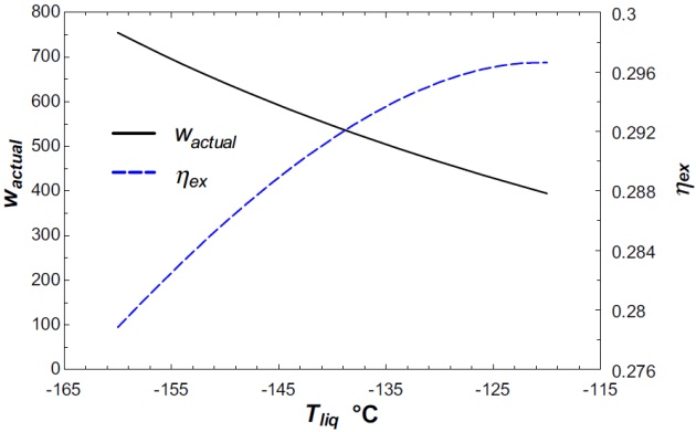
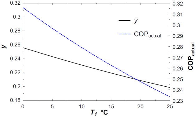
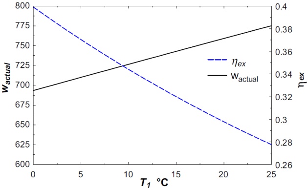
As part of the analysis, the effects of liquefaction temperature and gas inlet temperature on various energy- and exergy-based performance parameters are investigated considering the methane as the gas being liquefied. The results are given in Figures 14 to Figure 17. They show that as the liquefaction temperature increases and the inlet gas temperature decreases the liquefied mass fraction, the actual ​\( \style{font-size:22px}{COP} \)​, and the exergy efficiency increases while the actual work consumptions decreases.

Exergy losses in a nonideal Linde-Hampson liquefaction cycle

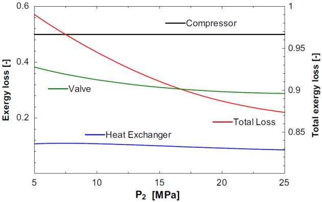
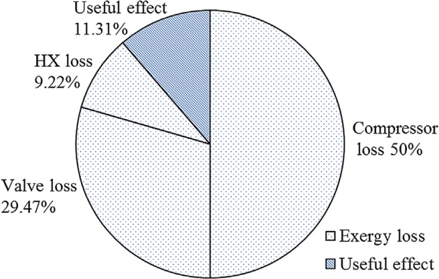
Consider the exergy losses in a nonideal Linde-Hampson methane liquefier. It can be assumed that the isothermal efficiency of the compressor is 60 %, and the effectiveness of the heat exchanger is 90 %. For the sake of simplicity, the pressure drop in the heat exchanger and phase separator is assumed to be zero. The compressor work is utilized in the liquefaction of methane and in overcoming the exergy losses in the compressor, heat exchanger, and valve. As shown in Figure 18, most of the exergy loss occurs in the compressor and then in the expansion valve even when the heat exchanger effectiveness is 90 %.

Compared to the ideal liquefier as discussed previously, the exergy efficiency is decreased from 27.67 to 11.31 % due to the irreversibility in the nonideal heat exchanger and compressor. Figure 19 shows the utilization of the input exergy in this nonideal cryogenic when high (​\( \style{font-size:22px}{P_2} \)​) and low (​\( \style{font-size:22px}{P_1} \)​) pressures are 25 MPa and 0.1 MPa, respectively.

Energy and exergy analyses of a nonideal Kapitza liquefaction system

A Kapitza liquefaction cycle has been shown schematically and on a temperature-entropy diagram in Figure 9, in order to describe energy and exergy analyses of liquefaction cycles. The fundamental difference between it and a Linde-Hampson liquefaction cycle is in the process used for expansion of the fluid from high to low pressure. Makeup gas is mixed with the uncondensed portion of the gas from the previous cycle, and the mixture at state 1 is compressed by an isothermal compressor to state 2. The temperature is kept constant by rejecting compression heat to a coolant. The high-pressure gas is further cooled in a first regenerative counterflow heat exchanger by the uncondensed portion of gas from the previous cycle to state 3, and then the main stream splits into two streams. One portion (9) passing through the expander undergoes a large temperature drop (10). This cold gas is used to cool and condense the high-pressure fluid in a second heat exchanger. The refrigeration obtained in the expander also helps in precooling the high-pressure methane in the first heat exchanger (HX-1) before it enters the expander and the second heat exchanger (HX-2). The high-pressure fluid is in a subcooled liquid state (5) at the entry of the throttle valve when the operating pressure (​\( \style{font-size:22px}{P_2} \)​) is lower than the critical pressure (​\( \style{font-size:22px}{P_c} \)​). The temperature of the high-pressure gas at the entry of the throttle valve is much lower than that in a Linde-Hampson system.

The expression for liquid yield (​\( \style{font-size:22px}y \)​) in a Kapitza liquefier is obtained by an energy balance over a control volume that excludes the compressor as follows:

\[ \style{font-size:22px}{y=\frac{h_{13}-h2}{h_{13}-h_f}+\frac{m\left(h_9-h_{10}\right)}{h_{13}-h_f}\;\;\;\;\;\;\;\;\;\;Equation\;52} \]

The first term on the right-hand side of the equation is the liquid yield in a simple Linde-Hampson liquefier. The second term represents the additional yield due to refrigeration effects from the expander. Thus, the refrigeration effect per unit mass of the gas in the cycle may be expressed as

\[ \style{font-size:22px}{q_L=h_{13}-h_2+m\left(h_9-h_{10}\right)\;\;\;\;\;\;\;\;\;\;Equation\;53} \]

where m represents the fraction of gas passing through the expander. The power extracted from the turbine ​\( \style{font-size:22px}{\left[m\left(h_9-h_{10}\right)\right]} \)​ can be used to reduce the compressor power in a Kapitza liquefier. The actual compressor input required in a Kapitza cycle can be written as

\[ \style{font-size:22px}{w_{atual}=h_2-h_1-T_1\left(s_2-s_1\right)-m\left(h_9-h_{10}\right)\;\;\;\;\;\;\;\;\;\;Equation\;54} \]

Similarly, the reversible work for Kapitza cycle may be expressed by the stream exergy difference of states 1 and 7 as

\[ \style{font-size:22px}{w_{rev}=y\left(ex_7-ex_1\right)=y\left(h_7-h_1-T_0\left(s_7-s_1\right)\right)\;\;\;\;\;\;\;\;\;\;Equation\;55} \]

Thus, the energy and exergy efficiency of a Kapitza liquefier can be expressed as follows:

\[ \style{font-size:22px}{COP=\frac{q_L}{w_{actual}}=\frac{h_{13}-h_2+m\left(h_9-h_{10}\right)}{h_2-h_1-T_1\left(s_2-s_1\right)-m\left(h_9-h_{10}\right)}\;\;\;\;\;\;\;\;\;\;Equation\;56} \]

\[ \style{font-size:22px}{\eta_{ex}=\frac{w_{rev}}{w_{actual}}=\frac{y\left(h_7-h_1-T_0\left(s_7-s_1\right)\right)}{h_2-h_1-T_1\left(s_2-s_1\right)-m\left(h_9-h_{10}\right)}\;\;\;\;\;\;\;\;\;\;Equation\;57} \]

Consider the exergy losses in a nonideal Kapitza methane liquefier. It can be assumed that the isothermal efficiency of the compressor is 5o %; the turbine adiabatic efficiency is 8o %; the minimum temperature approach is 1o °C in the first heat exchanger and 2o °C in the second heat exchanger. The operating pressure is assumed to be 4 MPa. Table 2 shows the thermodynamic parameters at different streams of the Kapitza methane liquefier.

Table 2. Thermodynamic Parameters of the Different Streams of a Kapitza Methane Liquefier
Stream	T [°C]	P [MPa]	h [kJ kg-1]	s [kJ kg-1 K-1]	e [kJ kg-1]	m [kg kg-1 gas]
1	25	0.1	-0.9762	0.004431	0	1
2	25	4	-40.01	-2.004	559.7	1
3	-33.64	4	-190.8	-2.568	577.1	1
4	-33.64	4	-190.8	-2.568	577.1	0.2344
5	-141.6	4	-835.6	-6.134	995.7	0.2344
6	-161.6	0.1	-835.6	-6.001	955.9	0.2344
8	-161.6	0.1	-911.5	-6.682	1083	0.1996
9	-33.64	4	-190.8	-2.568	577.1	0.7656
10	-161.6	0.1	-400.4	-2.098	227.5	0.7656
11	-161.6	0.1	-400.4	-2.098	227.5	0.9652
12	-72.84	0.1	-211.6	-0.85	44.16	0.9652
13	15	0.1	-23.18	-0.07132	0.3803	0.9652

 
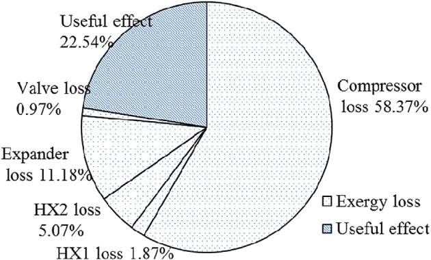
Figure 20 shows the utilization of input exergy in a Kapitza methane liquefier. It can be seen that the exergy loss in the throttling valve is only o.97 % in this case, compared to about 29 % in Linde- Hampson liquefiers. The smaller exergy loss in the throttling valve is due to the expansion of a subcooled liquid with a temperature change of about 2o°C, compared to the expansion of a superheated vapor with a temperature change of about iio°C. The exergy loss in the two heat exchangers and that in the expander are 11.18 % and 6.94 %, respectively. The exergy loss in the second heat exchanger is larger than that in the first heat exchanger, because the finite temperature difference in the HX2 is larger and also the temperature level is lower. The useful effect (exergy efficiency) of the Kapitza liquefier is 22.54 %, much higher than 11.31 % in the Linde-Hampson liquefier mainly due to the reduction of exergy loss in the throttling valve and compressor work input.

Pinch analysis

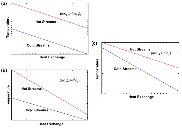
Figure 21 (a-c) shows typical temperature profiles of the hot and cold fluid streams in a counterflow heat exchanger with constant heat capacities but different relative values:

• (a) the same heat capacity of the hot and cold fluid streams;
• (b) larger heat capacity of the cold streams than that of hot streams;
• (c) larger heat capacity of the hot streams than that of cold streams.

Consequently, the minimum temperature approach between the streams occurs at the warm or cold end of the heat exchanger in Figures 21 (b) and 21 (c). In some cases, the specific heat of the fluids varies along the length of the heat exchanger, for instance zeotropic mixtures undergoing phase change or real fluids at temperatures close to the critical point when the pressure is greater than the critical pressure and critical temperature for all fluids. Thus, the minimum temperature approach between the hot and cold fluid streams of the heat exchanger may occur either between the two ends or at both warm and cold ends of the heat exchangers. The location where the temperature approach between the streams is at its minimum is called the pinch point.

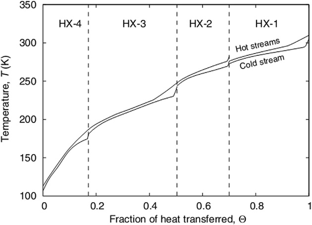
Figure 22 shows the temperature profile in the second heat exchanger (HX-2) in the Kapitza methane liquefaction process discussed in the previous section with operating pressures of 6/0.1 MPa. Pinch point occurs because of the large variation of the specific heat of methane at 6 MPa at temperatures close to the critical temperature of methane. 

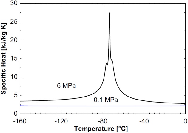
A large variation of the specific heat at constant pressure (​\( \style{font-size:22px}{c_p} \)​) with temperatures is observed in all real fluids at temperatures close to the critical point when the pressure ​\( \style{font-size:22px}P \)​ is greater than the critical pressure. The specific heat at constant pressure (​\( \style{font-size:22px}{c_p} \)​) tends to infinity at critical pressure and critical temperature for all fluids, as shown in Figure 23.

Pinch analysis is a methodology for minimizing energy consumption of chemical processes by calculating thermodynamically feasible energy targets (or minimum energy consumption) and achieving them by optimizing heat recovery systems, energy supply methods, and process operating conditions. It is also known as process integration, heat integration, energy integration, or pinch technology.

The process data is represented as a set of energy flows, or streams, as a function of heat load against temperature. These data are combined for all the streams in the plant to give composite curves, one for all hot streams (releasing heat) and one for all cold streams (requiring heat). The point of closest approach between the hot and cold composite curves is the pinch point (or just pinch) with a hot stream pinch temperature and a cold stream pinch temperature. This is where the design is most constrained. Hence, by finding this point and starting the design there, the energy targets can be achieved using heat exchangers to recover heat between hot and cold streams in two separate systems, one for temperatures above pinch temperatures and one for temperatures below pinch temperatures. In practice, during the pinch analysis of an existing design, often cross-pinch exchanges of heat are found between a hot stream with its temperature above the pinch and a cold stream below the pinch. Removal of those exchangers by alternative matching makes the process reach its energy target.

However, the major limitation with the heat pinch methodology is that only temperature is used as a quality parameter of a stream, thus neglecting pressure and composition. The advantage of exergy analysis is the inherent capability of including all stream properties (temperature, pressure, and composition). In a cryogenic liquefaction system (such as the Kapitza cycle discussed earlier), the temperature is closed related to both pressure and power, since compression and expansion (valve or turbine expander) will change the boiling and condensation temperature in order to be able to transfer heat from a cold source to a hot sink. The required energy (shaft work) and resulting refrigeration duty are determined by the hot and cold temperature levels, which dictates the required pressure increase or decrease and thereby the need for shaft work.

Aspelund et al. (2007) developed the Extended Pinch Analysis and Design (ExPAnD) methodology with particular focus on subambient processes to design a system of heat exchangers, expanders, and compressors in such a way that the irreversibilities are minimized for given a set of process streams with a supply state (temperature, pressure, and the resulting phase) and a target state, as well as utilized for external heating and cooling. They generalized the following conclusions based on general theoretical analysis:

1. Pressure-based exergy can effectively be transformed to cooling duty and work and may give a significant reduction in the required utility cooling for subambient processes;
2. Expanding a cold stream at high temperature will generate more work and cooling duty than at a lower temperature;
3. By heating the cold stream prior to expansion, more cooling duty will be produced and less irreversibility may occur in the heat exchanger, due to reduced driving forces;
4. Additional expansion steps and heat exchange passes may reduce the irreversibilities and create more cold duty and work;
5. If too much cold duty is produced, the heating requirement will increase and the driving forces will be reduced, however some additional work can be generated.

A set of detailed heuristics are introduced to utilize the ExPAnD methodology to design and optimize the subambient processes.

Some general heuristics:

1. Available pressure (​\( \style{font-size:22px}{P_s>P_t} \)​) can be utilized through expansion to reduce cold utility requirements with power generation as an important by-product. Contrary, lack of pressure (​\( \style{font-size:22px}{P_s<P_t} \)​) requires power; however, this situation may reduce hot utility requirements (​\( \style{font-size:22px}{P_s} \)​ and ​\( \style{font-size:22px}{P_t} \)​ denote the supply pressure and target pressure, respectively);
2. Temperature gap (​\( \style{font-size:22px}{\Delta_T>\Delta T_{min}} \)​) between the hot and cold composite curves results in unnecessary irreversibilities. The pressure of the streams may be manipulated to decrease the irreversibilities, generate power, and reduce the need for heating and cooling utilities. Streams with phase transitions are particularly suited for such manipulation.

Heuristics for streams with target pressure different from the supply pressure:

1. Compression of a vapor or dense phase stream requires power and will add heat to the system. Hence, from a Pinch analysis point of view, compression should preferably be done above the Pinch point;
2. Expansion of a vapor or dense phase stream in an expander will provide cooling to the system, and at the same time generate power. Hence, expansion should preferably be done below Pinch. In subambient processes, a stream with a supply pressure higher than the target pressure should always be expanded in an expander (not a valve) if the stream is located below the pinch point;
3. If expansion of a vapor or dense phase stream above Pinch is required, a valve should be used to minimize the increase in utility consumption, unless the main purpose of the expansion is to produce work.

Heuristics for streams with target pressure equal to the supply pressure:

1. A hot gas or dense phase fluid that is compressed above the Pinch point, cooled to near Pinch point temperature, and then expanded will decrease the need for both cold and hot utilities. Additional work is required, however.

Heuristics for liquid streams and streams with phase change:

1. A fluid with ​\( \style{font-size:22px}{P_s<P_t} \)​ should be compressed in a liquid phase if possible to save compressor work;
2. In a liquid stream with ​\( \style{font-size:22px}{P_s=P_t} \)​, a phase transition is necessary for the composite curves to be manipulated, since the effect of expansion/compression in the liquid phase alone is marginal;
3. If a cold liquid stream to be vaporized does not create a Pinch point, it should be pumped to avoid vaporization at a constant temperature, reduce the total cooling duty, and increase the pressure-based exergy. Work and cooling duty should be recovered by expansion of the fluid in the vapor phase at a later stage (higher temperature).

The ExPAnD methodology combines Pinch analysis and exergy analysis. It may be a very useful design tool for some cryogenic applications in which some of the heat exchangers are of the multistream type, enabling several streams with different entering and leaving temperatures to be joined in one heat exchanger, and expansion and compression work are involved to manipulate the temperatures of the hot and cold streams.

Energy and exergy analyses of natural gas liquefaction cycles

In this section, the energy and exergy analyses of three typical natural gas liquefaction cycles are discussed.

Propane-precooling mixed refrigerant cycle (C3/MRC)

Gu et al. reported a thermodynamic modeling and parametric analysis of a propane-precooling mixed refrigerant cycle (C3/MRC) based on the first- and second-law analysis. The schematic drawings of the mixed refrigerant cycle and propane-precooling cycle are shown in Figure 24 (a) and (b). The pressurized natural gas is precooled in the propane refrigeration unit, and then cooled down to the subcooled liquid state through three multistream heat exchangers.

Finally, it expanded to the ambient pressure at the throttle valve. Refrigerant mixture first is compressed to a high pressure of about 2.5 MPa in the two-stage compressor, and then is passed through a water cooler. It comes out at a temperature of about 305 K, and then is further cooled down in the propane refrigeration unit to about 238 K. Afterward, it comes through three multistream heat exchangers to provide the cooling capacity for liquefying supplied natural gas. In a propane-precooling refrigeration cycle, the propane experiences three-stage expansions, operating at three discrete evaporation temperature levels.

In the parametric effects on the cycle energy and exergy analysis, the following parameters and assumptions are given:

1. The process streams (e.g., natural gas) have an initial temperature of 298 K and pressure of 5 MPa with a flow rate of 1mol/s and with a composition of nitrogen (0.7 %), methane (82 %), ethane (11.2 %), propane (4 %), i-butane (1.2 %), and n-butane (0.9 %);
2. Liquefied natural gas is stored at the temperature of about 117.2 K and the pressure of about 0.15 MPa;
3. At the warm end of the first heat exchanger (HX-1), the refrigerant mixture has the composition of nitrogen (5 %), methane (44 %), ethane (34 %), and propane (17 %);
4. The heat transfer temperature difference at each end of the heat exchangers are assumed to be about 3 K;
5. The compressor efficiency is 0.75;
6. The high pressure of the propane-precooling cycle is about 1.3 MPa.

Table 3 summarizes the parametric effects on C3/MRC performances, and based on this case analysis some conclusions can be made as follows:

1. Natural gas feed pressure and the propane precooling temperature have relatively significant influences on the refrigerant mixture flow rate (​\( \style{font-size:22px}{q_{n,r}} \)​), total work input (​\( \style{font-size:22px}{W_{tot}} \)​), total refrigeration capacity (​\( \style{font-size:22px}{Q_{cmr}} \)​) and natural gas liquefaction (​\( \style{font-size:22px}{Q_{cng}} \)​) by MRC unit, and natural gas liquefaction by propane-precooling unit (​\( \style{font-size:22px}{Q_{cng}} \)​). Especially, increase of ​\( \style{font-size:22px}{Q_{cng}} \)​ is up to 16.35 %;
2. Natural gas precooling temperature ​\( \style{font-size:22px}{T_2} \)​ by the propane-precooling unit has the most significant effect on the required cooling capacity (​\( \style{font-size:22px}{Q_{png}} \)​); similarly for the effect of the suction temperature in MRC unit (​\( \style{font-size:22px}{T_9} \)​);
3. Compared to the high pressure (​\( \style{font-size:22px}{P_{13}} \)​), variation of the refrigerant mixture low pressure (​\( \style{font-size:22px}{P_9} \)​) affects total work input more significantly.

Table 3. Summary of Parametric Effects on C3/MRC Performances
Parameter Variation	Png(+31.58 %)	T2(+4.23 %)	T9(+2.79 %)	P9(+25 %)	P13(+5.04 %)
qn,r (%)	-6.83	+6.01	-3.59	+0.48	-2.16
Wtot (%)	-5.10	+3.86	-2.00	-5.34	-0.42
Qcmr (%)	-6.11	+5.41	-1.52	+0.71	-2.20
Qcng (%)	-6.88	+6.07	0	0	0
Qp (%)	-3.26	+1.53	-2.94	+0.40	-1.00
Qpng (%)	+16.35	-25.69	-9.19	0	0

 

Exergy analysis

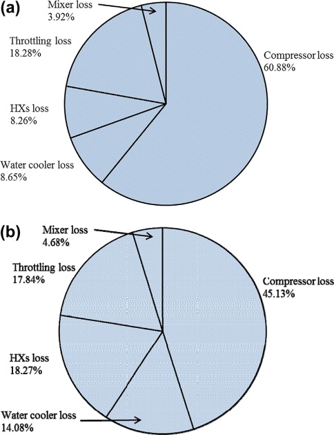
Based on the earlier parametric analysis, operating parameters of the C3/MRC cycle are determined, and therefore the corresponding analysis of exergy loss on each component of the entire cycle is performed. Figure 25 (a) and (b) show the relative exergy loss in the mixed refrigerant cycle (MRC) and in the propane (C3)-precooling cycle, respectively. It can be seen that for both cycles, the maximum exergy loss occurs in the compressord60.88 % for the MRC and 45.14 % for the C3-precooling cycle. In the MRC, the second highest exergy loss occurs in the throttling valves due to the significant amount of irreversibility in the isenthalpic expansion process. The results are those in the multistream heat ex-changers and water coolers after the compressor. Similarly, in the C3-precooling cycle the exergy loss in the throttling valve is also significant, although the second highest loss occurs in the multistream heat exchangers. For both units, the exergy loss in stream mixers is the lowest.

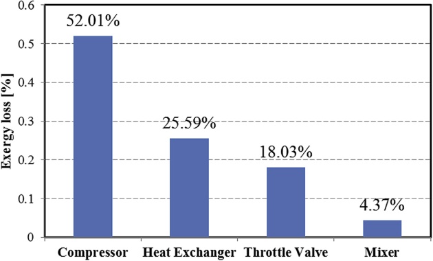
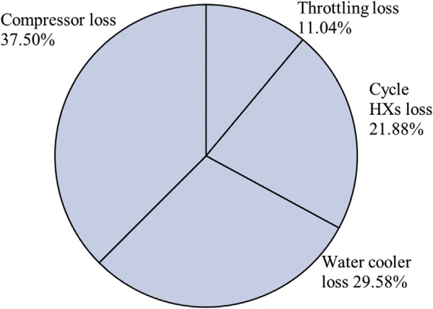
If comparing the exergy loss in the perspective of different types of process equipment in the entire natural liquefaction cycle, Figure 26 shows that the irreversibility in the compressors accounts for up to 52 % loss; the exergy loss in the heat exchange equipment is about half of that in compressors, 25 %; throttling loss in the expansion valves are about 18 %; the loss in all the stream mixers is only about 4 %.

According to the exergy analysis results, the possible directions to improve the cycle efficiency can be proposed as follows:

1. Choose the appropriate compressor suction temperature and compression ratio in the cycle design;
2. Improve the compressor design and therefore increase the compressor efficiency;
3. Utilize the heat transfer enhancement structure and increase the heat exchanger size to decrease the heat transfer temperature difference and irrepressibility;
4. Appropriately design the cycle to reduce the pressure drop in the throttling process or increase the subcooling of the process natural gas before the throttling process.

N₂-CH₄ expander liquefaction cycle

Pu et al. performed a thermodynamic analysis of ​\( \style{font-size:22px}{N_2-CH_4} \)​ expander natural gas liquefaction cycles. As a typical liquefaction process, the nitrogen expansion liquefaction cycle is a good option for small-scale liquefaction applications. The typical advantages and benefits of this process are its simplicity when compared with other liquefaction processes; adaptability to varied contents of feedstock by changing the composition of ​\( \style{font-size:22px}{N_2-CH_4} \)​ refrigerant mixture; certain requirement of refrigerant inventory and phase separators are eliminated since nitrogen and methane refrigerants are always in gas phase.

Two different cycles are considered in this case. The first process is single expander with a propane-precooling unit, as shown in Figure 27 (a). Adopting a propane precooling unit, which is a more efficient refrigeration method in the high temperature range, can consequently reduce the power consumption of the overall liquefaction cycle. The pressurized natural gas is cooled down to the subcooled liquid state through four multistream heat exchangers, and in the first heat exchanger (HX-1) natural gas is mainly precooled by the external propane refrigeration unit. In the ​\( \style{font-size:22px}{N_2-CH_4} \)​ expansion cycle, the mixture first undergoes two stages of compression during the compressor and the booster compressor driven by the refrigerant mixture expander. Then, the high-pressure refrigerant mixture is cooled first by using water coolers, and by the propane precooling unit in HX-1. Then it undergoes two different expansions in a expander and a throttling valve, respectively, to produce cold energy for HX-3 and HX-4.

Figure 27 (b) shows the second process with dual expanders in series. The first stage expander is used to produce cold energy at a high temperature range and thus to replace the propane precooling unit employed in the first process. By this means, no additional mechanical refrigeration is used, simplifying the process accordingly. But the associated penalty is to compress the ​\( \style{font-size:22px}{N_2-CH_4} \)​ mixture refrigerant to a higher pressure to produce greater cold energy, which in turn may increase the total power consumption. To make a fair comparison of two processes, the cold energy produced by the first stage expander is maintained the same as that produced by the propane refrigeration unit in the first process, which can determine the expansion ratio of the first stage expander. In this study, the following parameters and assumptions are made:

1. The feed natural gas has a temperature of 303 K and a pressure of about 0.2 MPa with a mass flow rate of 2.08 kg/s. It is liquefied and stored at the pressure about 0.12 MPa;
2. The minimum heat transfer temperature difference at each end of the heat exchangers is assumed to be about 3 K, and compressor and expander efficiencies are 0.7 and 0.78, respectively.

Effect of methane concentration in N₂-CH₄ refrigerant mixture

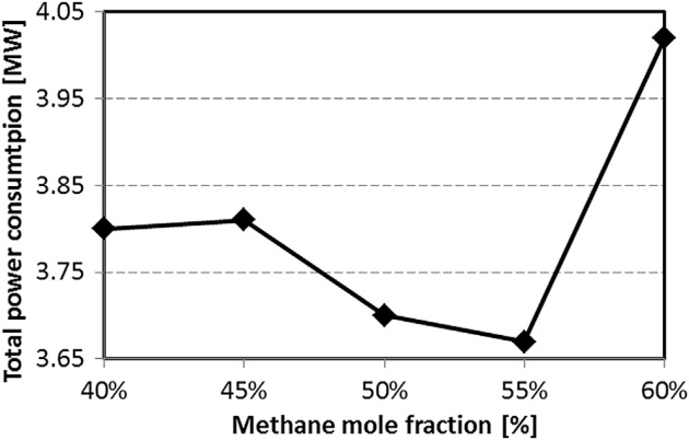
In both processes, the ​\( \style{font-size:22px}{N_2-CH_4} \)​ mixture is used as the working refrigerant to provide external cold energy for natural gas liquefaction. Methane and nitrogen are the high and low boiling point components, respectively. The methane mole fraction of the refrigerant mixture has two effects on the liquefaction cycle power consumption. The compressor work consumption per unit flow rate of the refrigerant mixture increases with the methane mole fraction. On the other hand, methane has a higher specific heat capacity than the nitrogen, thus the cold energy provided by the expander is greater per unit flow rate of the mixture with a higher methane concentration, which in turn will reduce the flow rate of the refrigerant mixture and possibly decrease the compressor power consumption. Figure 28 shows the effect of methane mole concentration in the refrigerant mixture on the total power consumption in the single expander cycle with a propane precooling unit at the same natural gas liquefaction rate. The power consumption reaches the minimum when the methane fraction is about 50 to 55 % for this case. In addition, Table 4 shows refrigerant temperatures before and after the throttling valve at varied methane mole fractions when the thermodynamic state after the throttling valve is fixed (P = 0.55 MPa, T = 105.15 K). It is clear that as the methane concentration increases, the refrigerant mixture must be precooled to a lower temperature before the throttling valve, and especially at 60 % the temperature begins to increase after the throttling. This indicates that the cold energy at a low tem-perature decreases when the mole fraction of the methane, high boiling point component, increases in the mixture. Based on this result, the mole fraction of the methane in the refrigerant mixture is chosen as 50 % in the following exergy analysis for both liquefaction processes.

Table 4. Temperatures of the Refrigerant Mixture before and after the Throttling Valve
Methane Mole Fraction [%]	Temperature Before Throttling Valve T14 [K]	Temperature After Throttling Valve T15 [K]
40	132	105.15
45	125.78	105.15
50	118.79	105.15
55	111.46	105.15
60	103.83	105.15

 

Exergy analysis

Figure 29 shows the relative exergy loss in each component for two different liquefaction processes. It can be seen that for both processes the compressor unit has the maximum exergy loss, up to about 42 %. Then, the results are the exergy losses in expanders, cycle heat exchangers, and throttling valves. In the first process, about 7.6 % exergy loss occurs in the additional propane refrigeration unit. Thus, it has only about 29.8 % exergy loss in the single-stage expander, about 10 % lower than in the dual expanders in the second process. Table 5 compares the power consumption in two liquefaction processes. Results reveal that the single expander cycle adopting a propane precooling unit saves about 5.5 % power consumption compared to the dual expander cycle.

Table 5. Power Consumption in Two Cycles
Main Components	The First Process [kW]	The Second Process [kW]
N2-CH4 compressor unit	3698.2	4624.5
Feed gas compressor unit	1508.6	1508.6
Propane precooling unit	589.5	–
Total power consumption	5796.3	6133.1

 
This is mainly due to the fact that the relatively large heat transfer temperature differences and the heat exchange load result in a significant amount of irrepressibility in the heat exchange process in the dual expander cycle.

Thus, the exergy efficiencies for two cycles are about 32.9 % and 31.0 %, respectively. It illustrates that the propane precooling unit is a more efficient refrigeration method in the high temperature range than the corresponding high temperature ​\( \style{font-size:22px}{N_2-CH_4} \)​ expander, and consequently reduces the power consumption of the overall liquefaction cycle. However, the dual expander cycle eliminates the conventional mechanical refrigeration unit. It is simpler and more compact, and thus requires less installation area, has greater safety, and is easier to operate. The dual expander may have more advantages than the propane precooling single expander cycle in certain applications that require high compactness and mobility such as offshore applications.

Cascade natural gas liquefaction cycle

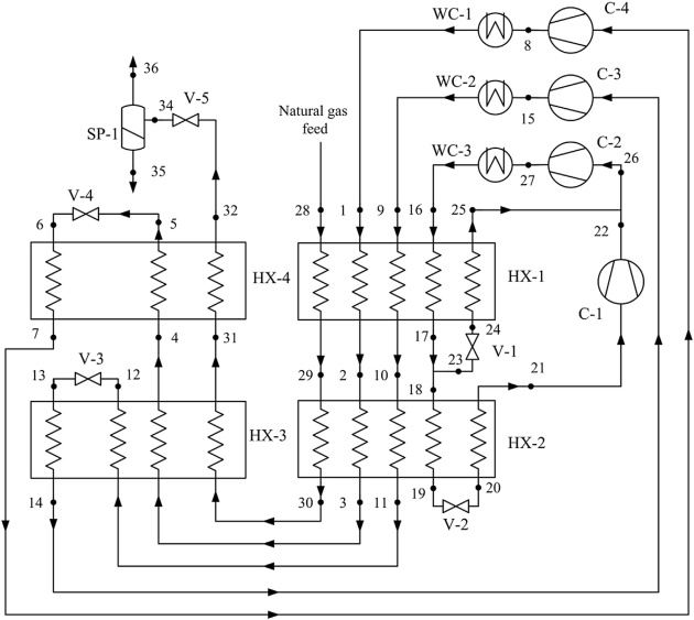
Figure 30 shows a patented cascade liquefaction process operating with refrigerant mixtures. It has three refrigeration stages with different refrigerants for each stage: one for desuperheating the natural gas feed, the second for condensation, and the third for subcooling. Consider the conventional cascade liquefaction process shown in Figure 30. The large number of phase separators and heat exchangers that need to be used makes the system quite complex.

Additionally, the main disadvantage with the conventional cascade process operating with pure fluid (single-component) refrigerants is that the refrigeration is provided at constant temperature at discrete temperature levels. On the other hand, mixed refrigerant processes provide refrigeration over a range of temperatures.

Table 6 shows the temperature, pressure, vapor fraction, and flow rate of different streams of the process. The precooling refrigerant (stream 16) is completely condensed in the condenser. All the other streams entering the first heat exchanger (HX-1) at the warm end are in a superheated state.

Table 6. Thermodynamic States of Different Streams in the Cascade Refrigeration Process
Stream	1	2	3	4	5	6	7	8	9
Temperature [K]	310	276.2	247.9	186.7	113.9	106.6	181.1	310	310
Pressure [MPa]	3.39	3.39	3.39	3.39	3.39	0.35	0.35	3.39	2.79
Vapor fraction [-]	1	1	1	0.297	0	0.109	1	1	1
Flow rate [mol/s]	0.721	0.721	0.721	0.721	0.721	0.721	0.721	0.721	1.023
Stream	10	11	12	13	14	15	16	17	18
Temperature [K]	276.2	247.7	191.5	180.9	242.7	326.1	310	282	282
Pressure [MPa]	2.79	2.79	2.79	0.31	0.31	2.79	1.69	1.69	1.69
Vapor fraction [-]	0.395	0	0	0.098	1	1	0	0	0
Flow rate [mol/s]	1.023	1.023	1.023	1.023	1.023	1.023	1.369	1.369	0.513
Stream	19	20	21	22	23	24	25	26	27
Temperature [K]	251	243.8	275.9	311.1	307.5	282	272.8	305.2	307.5
Pressure [MPa]	1.69	0.3	0.3	0.67	0.67	1.69	0.67	0.67	0.67
Vapor fraction [-]	0	0.054	1	1	1	0	0.077	1	1
Flow rate [mol/s]	0.513	0.513	0.513	0.513	1.369	0.855	0.855	0.855	1.369
Stream	28	29	30	31	32
Temperature [K]	300	276.2	247.9	186.8	113
Pressure [MPa]	6.5	6.5	6.5	6.5	6.5
Vapor fraction [-]	1	1	1	1	1
Flow rate [mol/s]	1	1	1	1	1

 
The high-pressure condensation refrigerant (stream 9) is condensed partially in the first heat exchanger and leaves the second heat exchanger (HX-2) as stream 11 in a subcooled state. On the other hand, the subcooling refrigerant (stream 1) leaves the third heat exchanger (HX-3) as stream 4 in a partially condensed state. All the low-pressure refrigerant streams enter the different compressors in a super-heated condition. Figure 31 shows the temperature of the hot and cold fluid streams in the four heat exchangers.

It can be seen that the temperature approach between the streams is small and nearly uniform throughout the length, except at temperatures close to the dew point temperature of the low- pressure refrigerant (cold) stream. This results in a relatively small log mean temperature difference. The small temperature difference between the cold and hot streams, particularly at low temperatures, significantly reduces the irrepressibility in the heat transfer process and results in a high exergy efficiency of the overall natural gas liquefaction process.

Figure 32 shows the exergy loss distribution in the overall process. The maximum exergy loss occurs in the compression units about 37.5 %, and it is lower than that in mixed refrigerant cycle (about 52 %). This is mainly because in the cascade cycle, each stream of refrigerant mixtures working at different temperature levels is compressed into different operating pressures. For instance, maximum pressures for the subcooling, condensation, and precooling refrigerants are 3.39 MPa, 2.79 MPa, and 1.69 MPa, correspondingly. Thus, the relative compressor work and irreversibility that occurs will be expected to be lower than that in the mixture refrigerant cycle where all the refrigerant mixtures are compressed to the same maximum pressure. Besides, the cascade cycle also has a relatively low cycle HX exergy loss compared to the ​\( \style{font-size:22px}{N_2-CH_4} \)​ expander cycle. As discussed earlier, this is mainly due to the relatively small and uniform temperature approach between hot and cold streams in the cycle HXs.

It is evident that for all the natural gas liquefaction cycles the combined losses for the compression system, including aftercoolers, are the most significant contributor to the work loss.

The work or exergy loss in this component is a direct result of the efficiency of the compression system and thus there is great potential to increase the cycle exergy efficiency by improving the compressor efficiency. In addition, for practical application, adopting a multistage compression system to split the compression system into multiple stages with intercooling will also help to reduce the compression work. In the case of the single expander liquefaction cycle, expander loss takes up to about 15.9 % of the total exergy loss. Any increase in the isentropic efficiency of the expander would reduce the required refrigerant flow rate since more cooling effect per flow rate will be generated in the expansion process, and also more useful work would be extracted to drive the generator or the compressor. Both effects would result in a power saving. For the heat exchangers system, using the mixed refrigerants will cause the lower exergy loss because the mixture composition can be optimized to minimize the heat transfer temperature difference between the hot and cold streams. Another option to enhance the cycle efficiency is to add a precooling refrigeration system since the same amount of refrigerating capacity will consume more power when generated at a lower temperature. But precooled liquefaction processes are preferable for large liquefaction systems.