Introduction
An essential part of any gas production operation is the accurate determination of volumetric flow rates. This is evident from all the material presented earlier in which almost all of the design procedures involve the determination of pressure loss for a particular flow rate. Therefore, unless accurate values for flow rate can be obtained, one cannot expect a system to perform according to its design.
This article presents the most common methods used in the field to measure gas flow rates. The orifice meter is by far the most widely used because of its simplicity, ruggedness, and accuracy. Application of orifice meters has been well documented in the past, and the standard reference is the American Gas Association Report Number 3. Other types of gas meters are briefly discussed, but their application is limited.
Most of the tables in this chapter are taken directly from the AGA Report 3. Many of the tables in the report are not included because the parameters tabulated involve only a simple calculation, and these properties can be obtained faster with a hand calculator than by referring to tables.
Orifice Metering
An orifice metering system consists of means for measuring the pressure drop caused by a change in velocity of the gas as it passes through a restriction placed in the pipe. The energy balance equation may be reduced to the following when all of the terms that do not apply are eliminated:
where conditions 1 and 2 refer to conditions in the pipe and conditions in the restriction or orifice, respectively.
Assuming that V1 = V2 = V, expressing the velocities in terms of flow rates, v = q/A and expressing the pressure change in head of flowing fluid results in:
where:
- q = volumetric flow rate;
- A2 = area of the orifice opening, πd22/4;
- β = d2/d1;
- g = acceleration of gravity;
- h = pressure drop across the orifice, head;
- d1 = pipe diameter, and;
- d2 = orifice or restriction diameter.
Equation 2 may be modified by specifying the pressure and temperature conditions at which the flow rate is measured, expressing h in inches of water and including a factor to account for the fact that irreversible losses were ignored.
where:
- qsc = gas flow rate at psc, Tsc, scf/hour;
- d2 = orifice size, in.;
- pf = flowing pressure, psia;
- Tf = flowing temperature, °R;
- hw = differential pressure across the orifice, inches of water;
- γg = gas specific gravity (air = 1), and;
- Ko = an efficiency factor.
Further modification is usually made by combining terms, assuming γg = 1, psc = 14,73, and Tsc = 60 °F to obtain:
where:
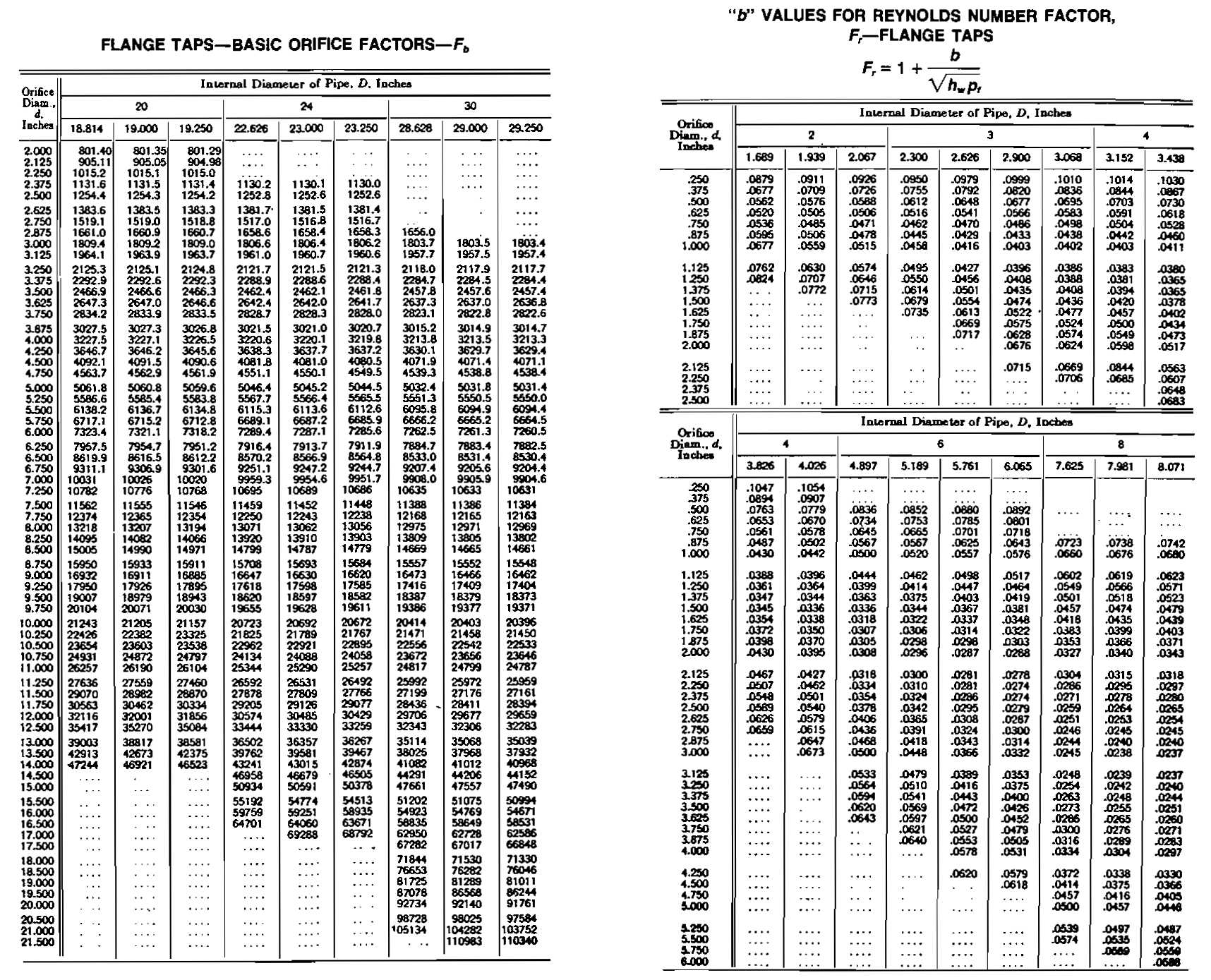
The term C ′ is known as the orifice constant, the value of which depends primarily on the basic orifice factor Fb = 338,17 Kod22. Many of the other terms are negligible or essentially equal to one. Values for most of these constants are tabulated for various orifice sizes and flowing conditions. The Fb factors are determined empirically and are periodically updated by the AGA.
Orifice Constants
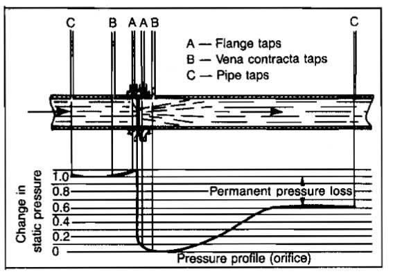
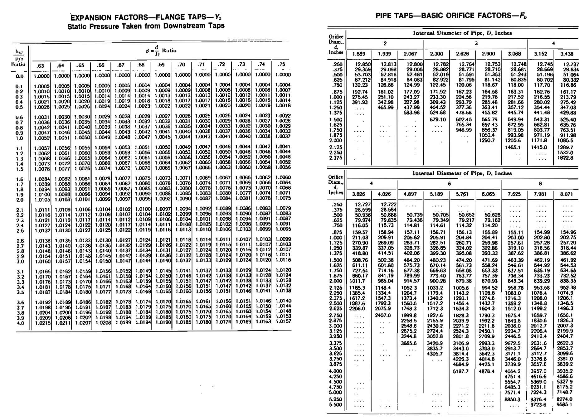
The values of the constants in Equation 5 depend on the points between which the differential pressure hw is measured. Two standards are provided in gas measurement-flange taps and pipe taps. With the former, the flange or orifice holder is so tapped that the center of the upstream and downstream taps is 1 in. from the respective orifice-plate surfaces. For standard pipe taps, the upstream tap is located 2-1/2 pipe diameters upstream and 8 pipe diameters downstream. The location of the taps makes an obvious difference in the values obtained. Tables are provided for both configurations. The relative locations of the taps are shown in Picture 1.
Basic Orifice Factor Fb. The Fb factor, as noted above, is based on those assumptions necessary to convert Equation 3 to 4.
These are:
- Tb = 520 °R;
- γg = 1,00 and;
- Tf = 520 °R.
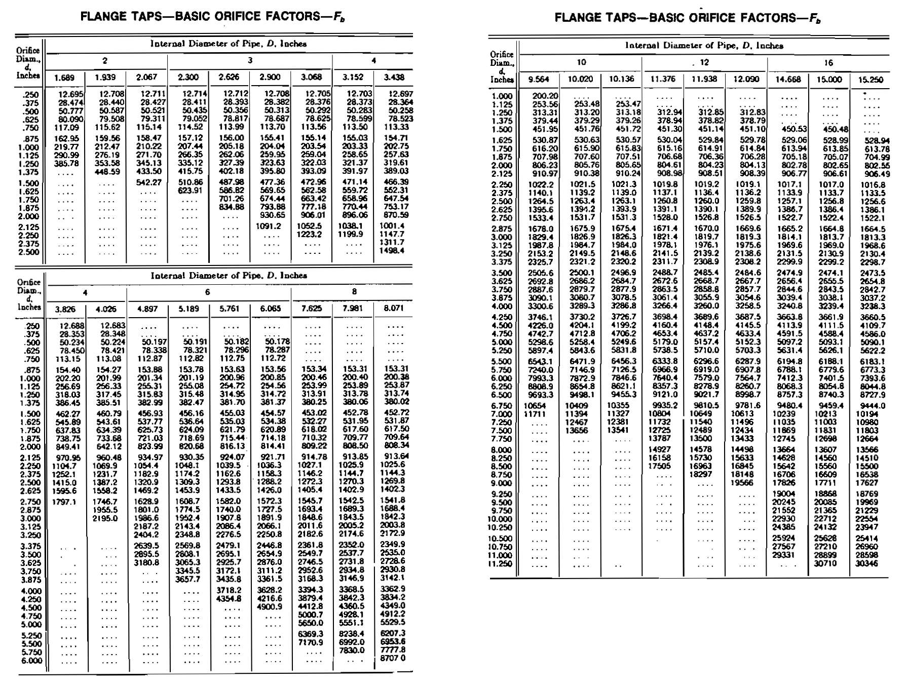
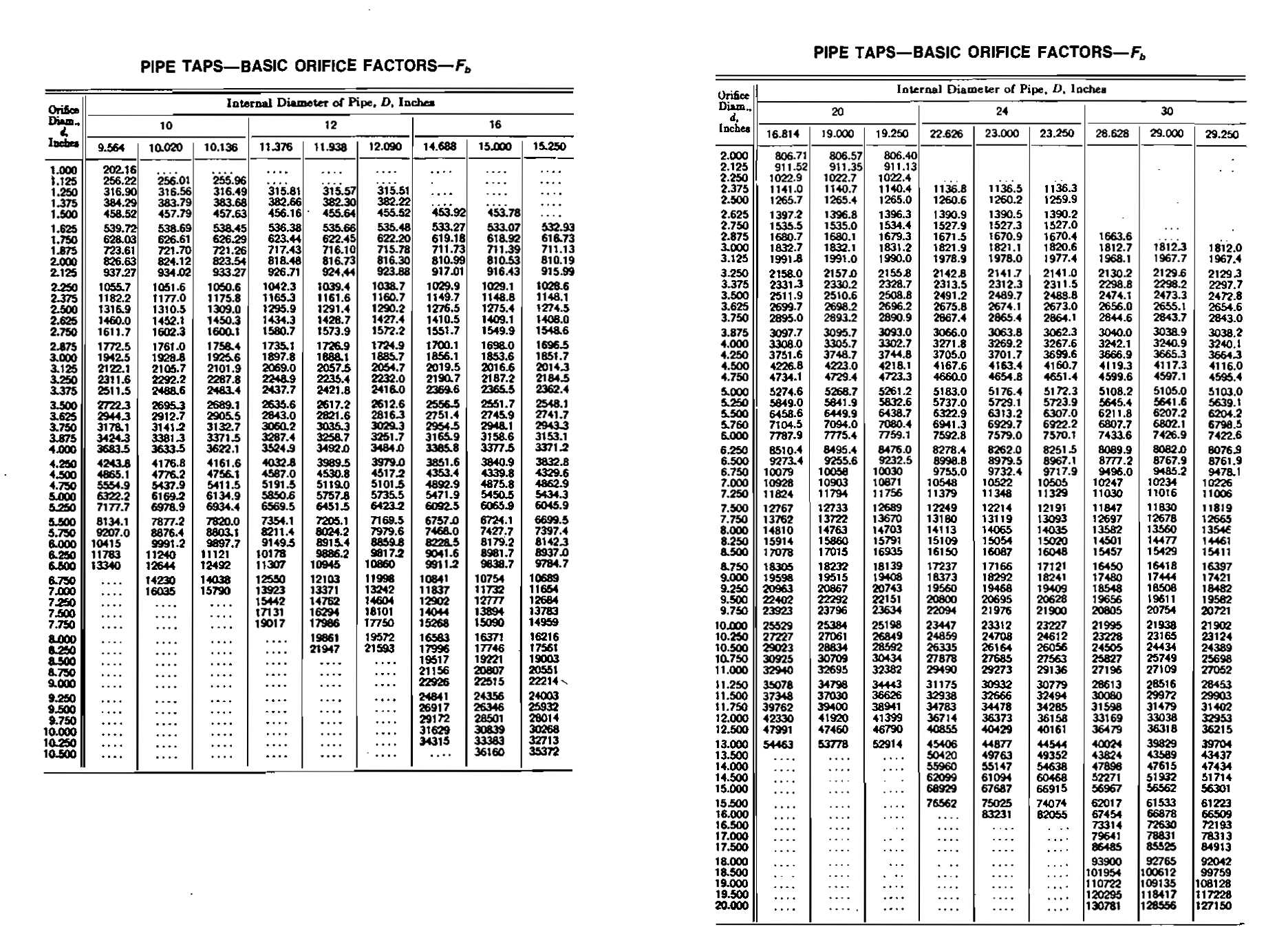
It is a function of the experimental Constant Ko which means that it depends on the location of the differential taps and the internal pipe diameter in addition to the orifice diameter. The value of Fb may be found from tables if the meter run is of standard internal diameter. For gas-measurement work involving sale and purchase by a gas-transmission or distribution company, corrections are provided for values of Fb not fitting the standard tables. These are not shown here, for they are not normally used in production operations. The charts show values of Fb for both flange and pipe taps.
Pressure-base Factor Fpb. The Fpb factor corrects the value of Fb for cases where the pressure base used is not 14,73 psia. It may be determined by the equation Fpb = 14,73/pb.
Temperature-base Factor Ftb. The Ftb factor corrects for any contract wherein the base temperature is not 520 °R (60 °F). This factor may be computed by the formula Ftb = Tb/520.
Specific-gravity Factor Fg. The Fg factor is to correct the basic orifice equation for those cases where the specific gravity of the gas is other than 1,00. The equation is Fg = γg-0,5.
Flowing-temperature Factor Ftf. The Ftf factor corrects for those cases where the flowing temperature of the gas is other than 60 °F. The equation is Ftf = (520/Tf)0,5.
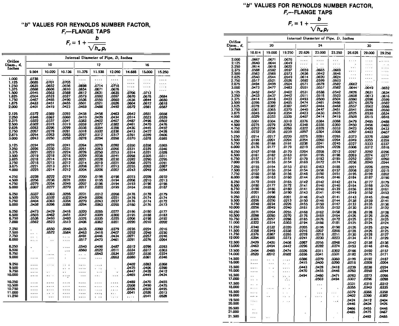
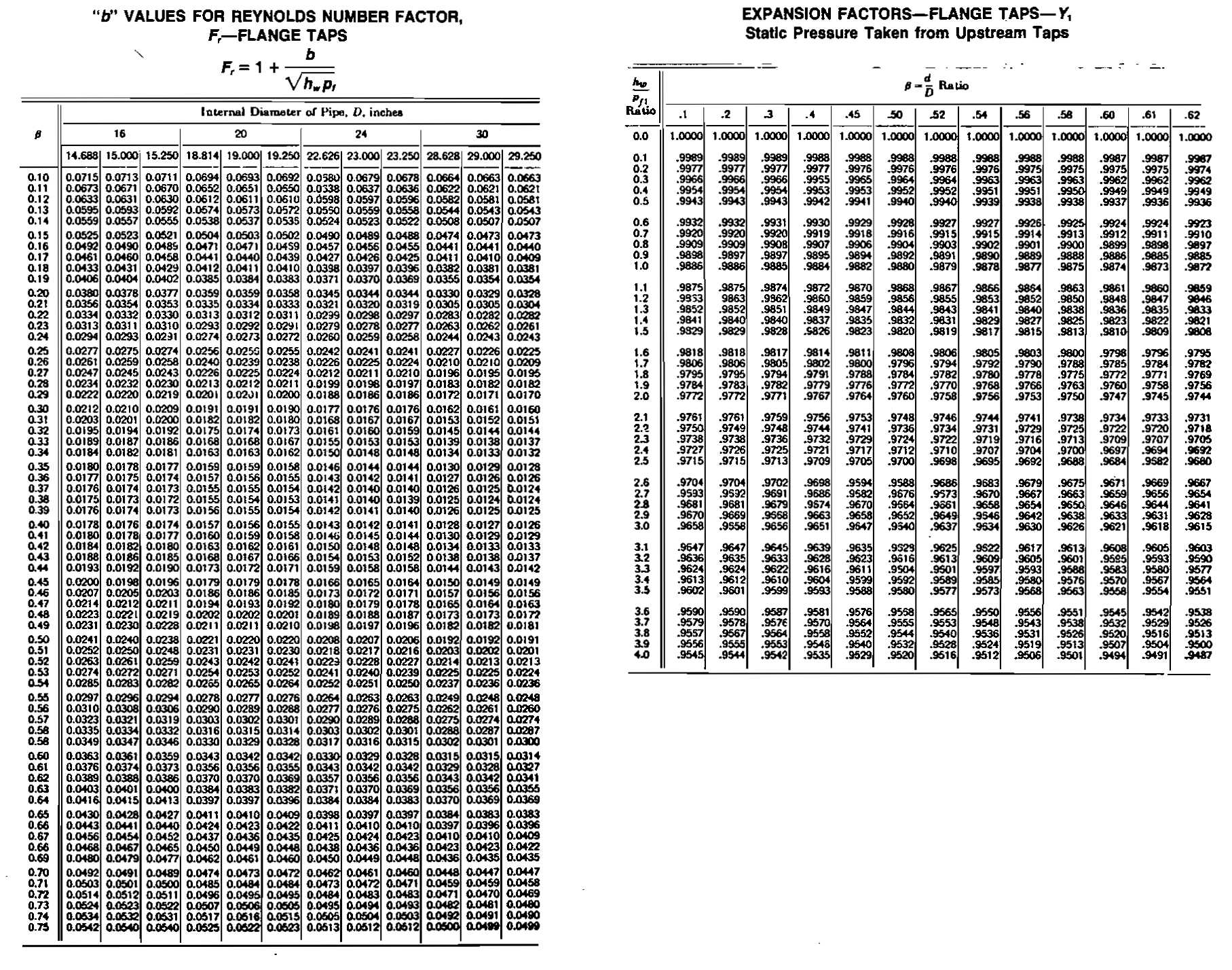
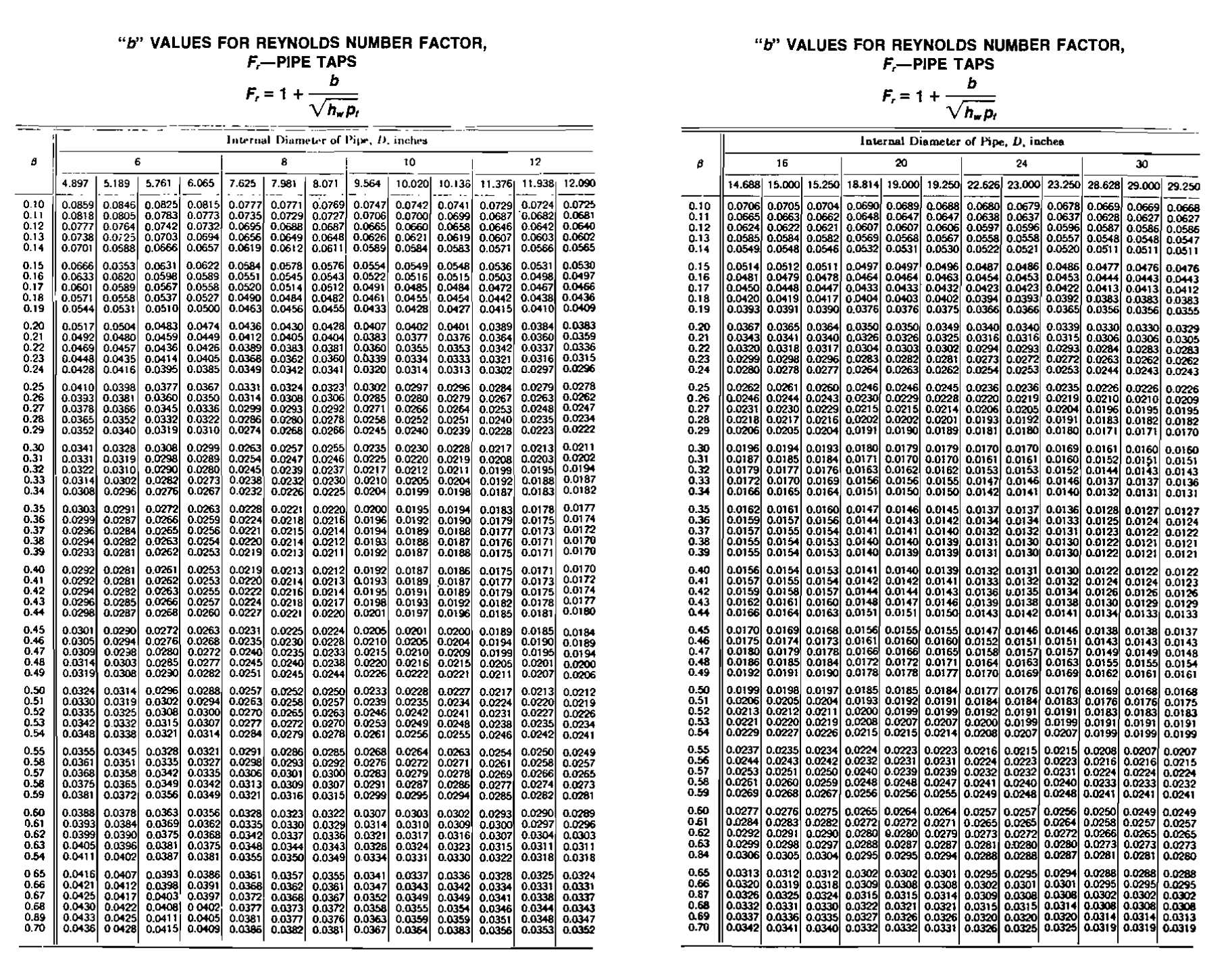
Reynolds-number Factor Fr. The Fr factor takes into account the variation of the discharge coefficient with Reynolds number. In gas measurement the variation is slight and is often ignored in production operations. Values are shown in the charts. It has been assumed in preparation of these charts that gas viscosity is substantially constant. The constant b shown in the charts is then primarily a function of pipe diameter, orifice diameter, and the location of the differential-pressure taps.
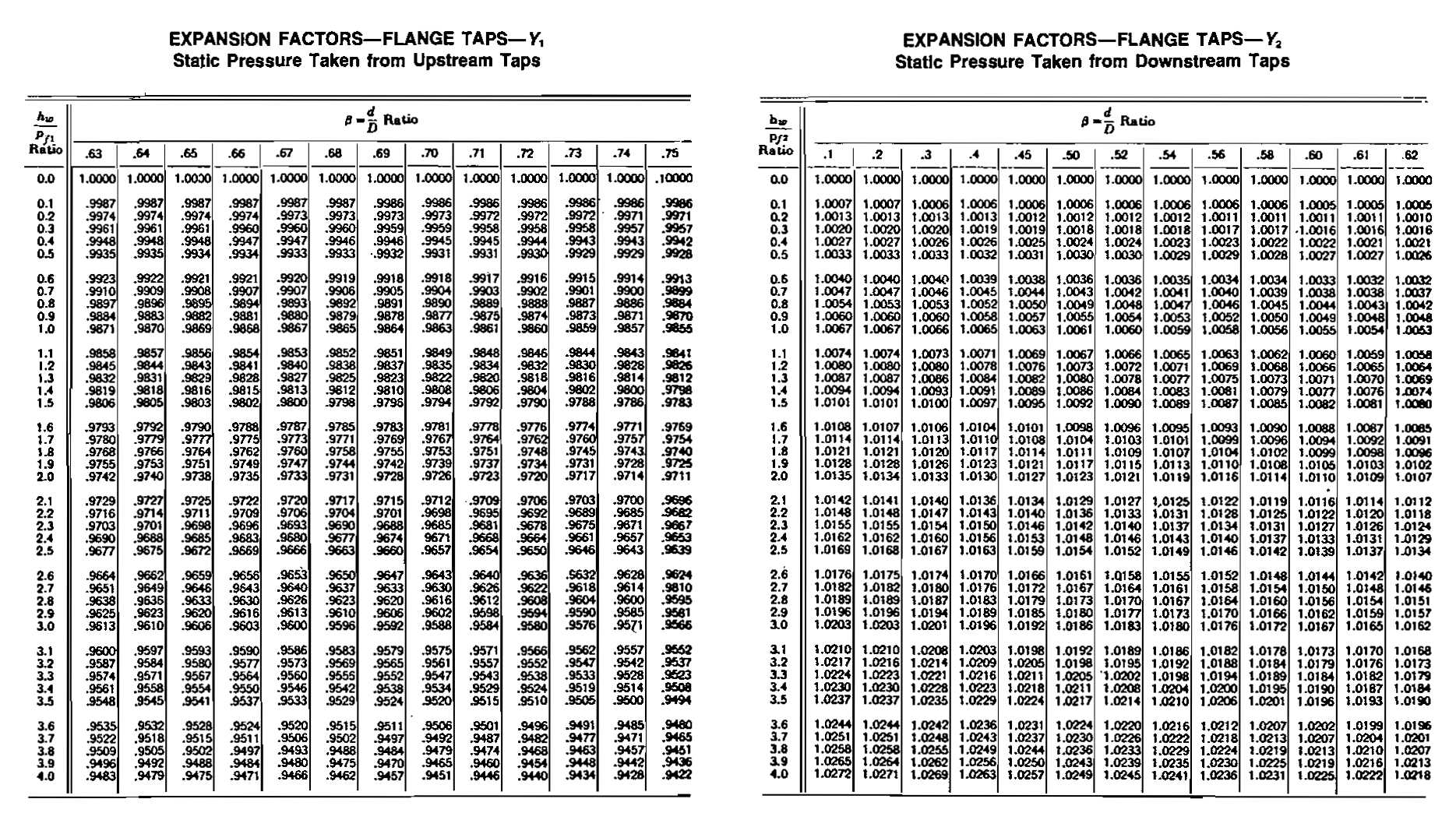
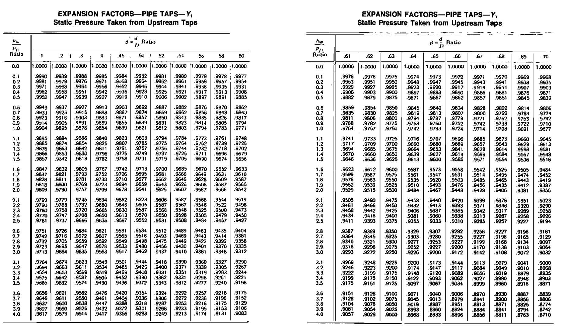
Expansion Factor Y. The Y factor accounts for the change in gas density as the pressure changes across the orifice. Inasmuch as the differential involved is usually small, this correction is small and often ignored. The value used depends on which of the differential-pressure taps is used to measure static pressure and the location of the tap. The additional primary variables involved are (1) β, (2) ratio of differential pressure to absolute pressure, and (3) the specific-heat ratio Cp/Cv. In the standard chart the last variable is taken as constant and equal to 1,3. Tables of this factor are shown in the charts.
Supercompressibility Factor Fpv. The variation from the ideal-gas laws of an actual gas is corrected by the Fpv factor. The factor may be measured experimentally or determined by detailed methods outlined in AGA Report 3. The correction is usually small and is often ignored. It may be estimated from the equation Fpv = (1/Z)0,5, where Z is equal to the compressibility factor obtained from standard correlations.
Manometer Factor Fm. The Fm factor is used only with mercury-type meters to correct for the slight error in measurement caused by having different heads of gas above the two legs of the manometer. For all practical purposes it is insignificant.
Metering System Design
Inasmuch as standard tables are used, careful attention must be paid to the physical setup of the metering system. Otherwise the results would vary with the installation.
Straightening Vanes. The purpose of straightening vanes is to minimize the effect of swirls, eddy currents, or irregular velocity distribution on meter accuracy. These vanes are built into a nipple and consist of a bundle of small pipe or tubing as shown in Picture 2.
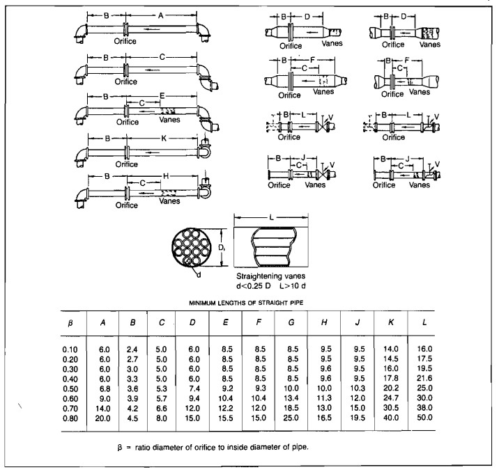
The diameter of each tube d should not exceed 1/4 the inside pipe diameter D. The length should be at least 10d. Unless necessary, vanes should not be used, since they are susceptible to erosion, introduce additional pressure loss, and clog easily.
Orifice Location. Picture 2 shows the minimum distance from valves and fittings that the orifice should be placed in order that proper metering might result.
Size of Orifice and Meter Run. The meter run should be sized so that the anticipated maximum and minimum flow rates may be handled within the satisfactory ratio of orifice to pipe diameter. In doing this it should be kept in mind that:
- The differential hw should not exceed the static pressure pf;
- The meter run ID should be at least one-third larger than the orifice opening;
- Both the differential and static-pressure pens should preferably operate within the middle 60 % of the recording chart range.
As a practical matter, the meter run ID should not be less than 3 in. in nominal diameter regardless of the small quantity of gas flowing. As a first approximation Equation 4 should be solved for C ′ at the flow rate, hw and pf desired. Then:
If the maximum anticipated flow rate is used to find C ′, multiplying the orifice size found in Equation 6 by 1,5 gives the approximate minimum pipe diameter needed. Once this has been established it is a relatively simple matter to change orifice plates as the flow varies to keep the values of hw and pf in the desired range.
Standard sharp-edged orifice plates should be used, the thickness of which is at least 1/16 in. For pipes larger than 4 in. the thickness of the plate should be at least 1/8 in. The thickness should not exceed one-eighth the orifice opening.
Recorder. The normal orifice meter is equipped with a two-pen recorder for measuring both static and differential pressure. The differential pen is normally actuated through a mechanical system using either a mercury manometer or a bellows. Both types are shown in Picture 3.
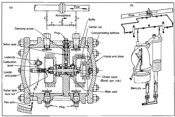
With the former a slight change in flow rate changes the level in the mercury manometer. A large float resting on the mercury changes level correspondingly and transmits this movement to the chart pen through a system of levers.
The bellows-type meter consists of two bellows filled with some fluid such as glycol. As the pressure differential changes this fluid moves between the bellows through a damping device, causing the bellows to expand or contract. The pen is actuated by a center rod that is connected to the free ends of the bellows. The small liquid-filled bellows located on the high-pressure side serves as an expansion device to correct for changes in ambient temperature.
Both types of instruments are equipped with check valves to protect them from differential pressures that exceed the range of the instrument. This is more of a problem with the mercury meter, since excessive differential pressure can blow mercury out of the meter, which destroys its calibration. In the bellows meter, soft-seated check valves prevent the flow of fluid between the bellows. Then the bellows are not likely to rupture since they are supported internally by the fluid contained within them.
The bellows meter has gained increasing popularity, particularly in field operations. Even though the initial cost is higher, many operators feel that this is compensated for by decreasing maintenance. It also offers the advantage of operating either properly or not at all, with little range in between. The problems of mercury loss and worrying about the change in calibration with the amount of mercury are eliminated. Until it fails, experience has shown that this meter needs little routine calibration.
With both types the static pressure is read from a pen actuated by a bourdon tube. The lead for this may come off either the upstream or downstream tap. In most installations it is good practice to install a bourdon tube having about twice the maximum pressure anticipated. This minimizes the problem of distortion, which destroys the original calibration of the tube. These tubes are available in many materials, the type depending on the service and the pressure rating desired.
Most meters are installed using a standard five-valve manifold of the type shown in Picture 4. One valve is placed on each of the leads to the pressure taps, two valves on the bypass, plus a vent valve. When the meter is placed in operation the bypass valves would be open, as would the two main valves, with the vent valve closed. The meter is then placed in service by slowly closing the bypass valves, followed by opening of the vent valve. This procedure prevents momentary pressure surges that might damage the meter or upset the calibration. The reverse procedure would then be used in taking the meter out of service. When the leads are bypassed the vent valve is an excellent place to obtain a gas sample.
Standard calibration procedure on the differential pen involves connecting one side of a water manometer into the high-pressure side of the meter. The low-pressure side of the meter is then opened to the atmosphere. This gives two manometers in parallel. By superimposing pressure on the high-pressure cell with a hand pump or similar device one may compare the meter reading with that of the manometer. If they are different the meter must be adjusted accordingly.
The bourdon tube may be calibrated simply by placing a dead-weight tester or a calibrated pressure gage in the lead line to the bourdon tube. By proper manipulation of the valves, the vent valve may be used to make this connection.
The circular charts used usually cover a time period of either 24 hours or 7 days. Many meters have clocks that may be easily adjusted for either time period. In most production operations 7-day periods are preferred, since this minimizes the cost of changing charts and the number of charts to be handled.
The charts used to record the static and differential pressures may be either the standard type, which record directly the values of hw and pf or the square root or L-1O type, which record the square root of the static pressure and differential pressure. Since the zero reading on the L-1O chart corresponds to zero pounds absolute, the pressure pen must be set at local atmospheric pressure. The position of the pen for zero gage pressure (atmospheric pressure) depends on the atmospheric pressure and the range of the static spring in the recorder. It may be calculated from:
where:
- pzero = pen setting for zero line pressure, psi;
- pa = local atmospheric pressure, psia, and;
- Rp = pressure range of meter, psi.
The actual scale of the L-10 charts is from zero to ten; therefore, the correct values of static and differential pressures depend on the ranges of the static and differential springs in the meter. The actual flow rate is calculated from:

or:
where:
- qsc = flow rate, scf/hr;
- Rh = range of differential element, inches;
- Rp = range of static element, psi;
- C ′ = orifice constant (Eq. 5);
- hu = chart differential reading;
- pu = chart static reading, and;
- , which is constant for a particular meter.
Example 1:
A meter run that is equipped with flange taps and a 3,000 inch orifice has an inside diameter of 6,065 inches. The static pressure, obtained from the downstream tap, reads 80 psia and the average differential pressure is 49,5 inches of water. If the pressure and temperature bases are 14,9 psia and 60 °F respectively, calculate the flow rate in cubic feet per hour. The gas specific gravity is 0,60 and the flowing temperature is 65 °F.
Solution:
1 Calculate C ′ = Fb Fpb Ftb Fg Ftf Fr Fpv Fm Y. From the tables. for:
- d = 3,000 and;
- D = 6,065;
- Fb = 1891,9.
From the tables, b = 0,0332,
For γg = 0,6, T = 65 F, p = 80 psia, the value calculated for Z is 0,990.
To determine Y:
From the tables, Y = 1,0037 (requires interpolation).
2 Calculate qsc:
Example 2:
A metering system is required to measure approximately 8,5 MMscfd of 0,62 gravity gas at a line pressure of 250 psig. The meter run is to be made of 8 in. pipe (7,981 in. ID). Determine the size of the orifice plate to give a differentiai of about 50 inches. Flowing temperature averages about 80 °F.
Solution:
For:
For an approximation, all of the terms in Equation 5 except Fg and Ftf can be Ignored in this case. Therefore:
From the Fb tables for flange taps, for D = 7,981 one obtains:
| d | Fb |
|---|---|
| 3,375 | 2 352,0 |
| 3,500 | 2 537,7 |
Therefore, a 3,500 inch orifice plate would be selected to obtain an hw reading of approximately 50 inches at the design flow rate.
Example 3:
The metering system described in Example 1 is equipped with an L-10 recorder that has a differential element range of 100 inches and a static element range of 250 psi. Calculate the flow rate if the following readings are obtained:
- hu = 7,00;
- pu = 5,7.
Solution:
From Example 1, C ′ = 2 426,9
Chart-Reading Accuracy
In most cases when charts are obtained from the field the values of hw and pf or hu and pu will not be constant for the entire period covered by the chart. It then becomes necessary to either divide the chart into small enough increments such that the readings can be considered constant or to use integrating devices to obtain the cumulative flow in standard cubic feet for the total chart period.
Various devices are used to mechanically compute the total flow from the chart records, reducing the work required to obtain such a figure from a visual inspection of the chart. Some of these devices are quite complex and expensive but are inherently more accurate.
The simplest device is the linear, or averaging type, planimeter. This instrument merely obtains the area under the curve corresponding to one of the chart records. Consequently, this record could only be used to obtain an average value for the chart record integrated. Since flow varies as the square root of that record in absolute units, the preferable value would be the average square root-instead of being the square root of a direct average. The average square root and the square root of the average value are quite close if the record is fairly constant.
A somewhat more complex instrument is available in the form of a planimeter fitted with a calibrated actuating cam that extracts the square root of the chart reading. This square root planimeter is intended for use with L-10 charts. Traversing the circle corresponding to line 7 will result in a reading of 7,00 for a complete chart revolution; a reading of 3,00 will be obtained from tracing a circle corresponding to line 3, etc. This instrument gives a fundamentally more correct analysis of the chart records-being correct, within the limits of measurement, as long as one of the chart records is constant to within 10 %. This is the limitation normally put on this instrument. For gas or steam being measured at constant pressures, or in the measurement of liquids, the results obtained with a square root planimeter are theoretically correct.
To obtain a theoretically correct integration, when both chart records vary considerably, the integration must be performed on both records simultaneously. An integrator of this type is inherently more complex and expensive, but its use is justified when the number of charts to be processed is quite large. Such an integrator fulfills the theoretical requirement that the integration be a summation of the square roots of the products of the pen readings, which necessitates the simultaneous integration of the chart records. The integration involves the absolute static pressure, and since most chart records give this variable as a gage pressure, it is necessary to make an adjustment on the arm of the pen that traces the static pressure record to account for the average barometric pressure.
Conditions Affecting Accuracy
Various conditions can exist in the field that adversely affect the measuring accuracy of an orifice metering system. It is common practice to install a metering system and then to accept the results as long as no obvious malfunctions occur.
Condition of the Orifice Edge. The greatest source of error in the primary measuring elements is probably the possible deviation from the specification that the up-stream edge of the orifice plate be square and sharp. A slight rounding of the edge can produce a considerable increase in the discharge coefficient, which results in low measurement. This is especially true with the smaller orifices in the smaller line sizes since the effect of the edge imperfection is relative. A wire-edge burr, or fin, on the orifice edge is also undesirable since it can alter the flow pattern of the stream from that corresponding to proper measurement.
Condition of the Meter Tube. Some error can be introduced as a result of a variation of the finish of the inside of the meter tube. The accepted orifice discharge coefficients were obtained from tests with meter tubes constructed of commercial iron pipe with the corresponding inside surface roughness. Too smooth an inside surface can introduce a slight error in the measurement, just as an error can be produced by too rough a surface, since either condition constitutes a deviation from the conditions under which the accepted discharge coefficients were determined. Measurement would be high with too smooth an inside pipe surface and low with too rough an inside surface.
Pulsation. The effects of pressure and velocity pulsations in the vicinity of the orifice constitute a very indefinite phase in the measurement of gas with an orifice meter. This pulsation can be of a low frequency form such as might result from reciprocating compressors, undamped pressure regulators, chattering valves, or liquid surging back and forth at low points in the line. It might also be a high frequency pulsation caused by resonance of the pipe lines themselves. The pulsations of lower frequency probably have a greater effect on the measurement; however, no conclusive information is at present available by which the pulsation errors can be completely correlated with pulsation frequency or with the wave form and amplitude of those pulsations. This problem has been recognized; considerable research is under way to determine means of either eliminating the effect of pulsations or to determine the degree of error that the pulsation might produce.
In some instances, the effect of pulsation has been largely reduced by installing restrictions in the line that produce pressure drops up to 10 % of the line pressure. In many cases, resistances that create much smaller pressure drops have been found satisfactory. In other instances, the effect has been minimized by installing volume tanks, baffles, or dampeners in the line. When any of these devices are used they should be installed between the meter tube and the source of the pulsation.
Other problems can be created by operations that might be employed to obtain a smoother chart record, such as pinching gage lines or over-damping a meter. None of these operations eliminates the basic error corresponding to the pulsation in the line. Pinching gage line valves might even increase the error in the measurement. Furthermore, the pulsation might be of sufficiently high frequency so that, even with an undamped meter, the instrument pens would not follow the fluctuations. Under these conditions a considerable error might exist without any visible indication on the instrument. Probably the best policy would be to install the meter at a point as remote as possible from the source of any pulsation.
In summary, to obtain reliable measurements, it is necessary to suppress the pulsations. The following items, in general, are valuable in diminishing pulsation and/or its effect on orifice flow measurement.
- Locating the meter tube more favorably with regard to the source of pulsation such as at the inlet side of regulators, or increasing the distance from the source of pulsation.
- Inserting capacity (volume) or specially designed filters in the line between the source of pulsation and the meter tube in order to reduce the amplitude of the pulsation.
- Operating at differentials as high as is practical by installing a smaller orifice or by concentrating flow, in a multiple tube installation, through a limited number of the tubes.
- Using smaller-sized tubes and keeping essentially the same size of orifice, while still maintaining the highest practical limit on the differential.
Effect of Water Vapor. In the measurement of gas containing moisture in a vapor state, the effect of the moisture depends largely on the specific gravity of the gas. Natural gas is quite dry, and its specific gravity is usually quite close to that of the water vapor, about 0,62. For this reason the only appreciable correction would be a direct volume correction based upon the partial pressure of the water vapor at flowing conditions.
In the measurement of certain gases of known composition, the specific gravity is often calculated from the molecular weight or is determined from a moisture-free sample. Under these conditions, especially with very light or very heavy gases, a correction must be made for the erroneous specific gravity obtained by having neglected the moisture content of the gas.
Wet Gas Measurement. The effect of liquid in the gas stream on measurement is a problem that has never been completely solved. Various arrangements of meter tubes, gage line piping, and drip pots have been used in an effort to minimize the errors resulting from liquid accumulating ahead of the orifice plate, at low points in the gage lines, or in the chambers of the meter manometer. An accumulation of liquid ahead of the orifice plate disturbs the normal flow pattern and alters the discharge coefficient for the orifice. Liquid trapped in the gage lines distorts the differential pressure and causes the manometer to give an incorrect indication. Liquid in the chambers of a mercury manometer can cause an unbalance that will alter the zero setting of the instrument by introducing a “wet-leg” or condition of unbalance, in the manometer. Bellows-type manometers, with gage lines attached to the bottom of the manometer chambers, are self-draining and, therefore, eliminate that portion of the error corresponding to the liquid that might find its way into the manometer. With bellows-type meters no error results from liquid being in the manometer chambers, because of a “wet-leg” effect. There would be an error, however, if a difference in liquid levels existed in the manometer chambers, or in the gage lines, under conditions of partial flooding. With either type manometer it is recommended that the manometer be installed above the line, that 1/2 in. (or larger) gage lines be used, and that the gage lines be well graded to permit drainage of liquid back into the meter tube.
The effect of the mechanically entrained liquid that flows through the orifice in the form of a mist is a subject of considerable conjecture. It is difficult to determine anything other than an average value for the amount of liquid entrainment such as might exist over a period of days or weeks. Such an average indication and the corresponding density increase might be obtained from ratios of barrels of liquid per million cubic feet of gas, etc. There is some question, however, as to whether the flow actually varies in strict accordance with the change in average density.
The common practice has been to determine an average density for the mixture and presume that the flow rate corresponds to a fluid of that density.
Other Metering Methods
For well-test purposes other forms of velocity meters are used:
- Orifice well testers;
- Critical-flow provers and;
- Pitot tubes.
These methods are not as accurate as the meters discussed above but are convenient and often yield results accurate enough for the purpose.
Orifice Well Tester
The orifice well tester consists of a 2-in. nipple with provision for attaching different sharp-edged orifice plates on the end. The static pressure just upstream from this plate may then be measured. The accuracy of this device is limited but it is suitable for measuring the amount of gas being produced where the pressures are relatively low and the production is to the atmosphere.
Tables for converting the meter reading to flow rates are provided with the meter and may differ among manufacturers.
Critical-flow Prover
The critical-flow prover is a device that also exhausts the gas to the atmosphere. It is also a special pipe nipple with a flange for holding special plates to the end. It is based on the principle that the velocity of sound represents the maximum speed at which a pressure effect may be propagated through a gas; i. e., once this velocity is reached further increase in the pressure differential will not increase the pressure at the throat. This means that the mass rate of flow would not increase as the pressure ratio p2/p1 was decreased below this critical value. With ideal gases the critical ratio is 0,49 for monatomic gases and 0,53 for diatomic gases, with slightly higher values for complex gases. Saturated steam, for example, shows a critical pressure ratio of 0,55. The range of these values is the source of the common rule of thumb that once the pressure reduction is twofold critical-flow phenomena limit the mass rate of flow.
When metering gas under such conditions the volume rate of flow will be a function of upstream pressure, gas gravity, and gas temperature since it is a compressible fluid.
The orifice used differs from that in the orifice meter. It is thicker and has a rounded edge. This edge is placed toward the flow, since experience has shown that a sharpedged orifice does not give reproducible results under critical-flow conditions. In fact sharp-edged orifices do not conform to existing theories and correlations. The general equation for a critical-flow prover is:
where:
- p = pressure on prover, psia;
- C = orifice coefficient for prover;
- qsc = rate of flow, (Mcf/D), measured at 14,4 psia and 60 °F;
- γg = specific gravity of gas (air = 1,00), and;
- T = absolute temperature, °R.
The critical-flow prover is one of the basic devices used for determining the gas flow rate in the open-flow testing of gas wells. Values of the coefficient C may be found in Table 1.
Pitot Tube
The pitot tube is another measuring device used extensively during preliminary well tests. It works by measuring the difference between the impact pressure at the tip and the static pressure in the flowing stream. This impact pressure results from conversion of the kinetic energy of the flowing gas to pressure. If the conversion efficiency is relatively constant a conversion between pressure and flow rate is possible. The pitot tube is normally made of 1/8-in. ID pipe and is inserted in the center of a nipple at least 8 diameters long.
| Table 1. Orifice Coefficient for Critical-Flow Provers | ||
|---|---|---|
| Size of Orifice, in. | Orifice Coefficient | |
| 2-in. Prover | 4-in. Prover | |
| 1/16 | 1,524 | |
| 3/32 | 3,355 | |
| 1/8 | 6,301 | |
| 5/16 | 14,47 | |
| 7/32 | 19,97 | |
| 1/4 | 25,86 | 24,92 |
| 5/16 | 39,77 | |
| 3/8 | 56,68 | 56,01 |
| 7/16 | 81,09 | |
| 1/2 | 101,8 | 100,2 |
| 5/8 | 154,0 | 156,1 |
| 3/4 | 224,9 | 223,7 |
| 7/8 | 309,3 | 304,2 |
| 1 | 406,7 | 396,3 |
| 1 1/8 | 520,8 | 499,2 |
| 1 1/4 | 657,5 | 616,4 |
| 1 3/8 | 807,8 | 742,1 |
| 1 1/2 | 1 002 | 884,3 |
| 1 3/4 | 1 208 | |
| 2 | 1 596 | |
| 2 1/2 | 2 566 | |
| 3 | 3 904 | |
A pitot tube is used largely for temporary flow measurement since it is small and easy to handle. Very few permanent installations are made, since it produces low-pressure differentials, is difficult to calibrate, and often clogs.
A pitot tube measures a point velocity, i. e., the velocity at only one point across the cross-section of the pipe. In the absence of unknown disturbing elements such as pipe burrs or undue roughness, the velocity at the center is theoretically 20 % greater than the mean velocity. For approximate measurement, standard tables use this factor to convert readings taken at the center of the pipe to a volume flow rate. For exact work the mean velocity would be found by taking a series of experimental velocity measurements across the pipe diameter.
A similar method is used for large gas-flow rates and/or where debris produced with the gas makes other methods unfeasible. This method consists simply of measuring the static pressure through a side opening 4 diameters from the end of a nipple at least 8 diameters long. This is the least desirable of the methods discussed because of the potential error involved. Further data on the use of these devices for the measurement of gas flow may be found in U. S. Bureau of Mines Monograph 7.
Turbine Meters
A turbine meter is a velocity responsive meter that is connected in the pipeline such that the entire gas stream passes through the meter. A propeller in the meter turns at a velocity which is proportional to the velocity of the fluid flowing through it. The secondary element may be a revolution counter or other means of sensing and totalizing the revolutions of the propeller or rotor. Turbine meters have been more widely used for measuring liquid flow than gas flow because the driving torque for the rotor depends on the density and the square of the fluid velocity. Therefore it is necessary to have the resisting torque very low for gas measuring; yet it is necessary that this torque be constant throughout the operating range of the meter.
The range of flow rates that can be handled with a turbine meter depends on the size of the meter, the density of the fluid and the viscosity of the fluid. The normal range is about 10 to 1 with an accuracy band of plus or minus 0,5 %. Turbine meters used for gas measurement are usually calibrated with a critical flow prover or with an orifice meter of known accuracy. Velocity fluctuations occurring in a turbine meter, caused by turbulence or pressure fluctuations, will cause a turbine meter to register too high.
Table 2:


Although the orifice meter is certainly the most commonly used device for measuring large quantities of gas, various other types of meters have been proposed or are in the development stage presently. Other than those already discussed are the magnetic flowmeters, thermal meters, anemometers, current meters, vortex shedding meters, and sonic flowmeters.