LNG plants are massive energy consumers. This is due to the fact that the energy required for liquefying one kilogram of natural gas is around 1,188 kJ. However, this liquefaction energy varies depending on the liquefaction cycle and site conditions. Practically about 8 % of the feed gas to the LNG plants is consumed for the liquefaction. Most of the LNG plant energy consumption occurs in the compressor drivers where fuel energy (usually natural gas) is converted to mechanical work (or electricity in case of electrically driven compressors). Due to the energy consumption scale of the LNG plants, any enhancement to the energy efficiency of LNG plants will result in a significant reduction in gas consumption and consequently \( \style{font-size:22px}{CO_2} \) emission.
There are two ways to increase the energy efficiency of natural gas liquefaction cycles: liquefaction cycle enhancement and driver cycle enhancement. Liquefaction cycle enhancements reduce the compressor power and consequently the compressor driver’s fuel consumption. Driver cycle enhancement reduces the amount of fuel consumption to generate a specific amount of power. Typical natural gas liquefaction cycles utilize either pure refrigerant in cascade cycles, expansion-based cycles, or mixed refrigerant cycles. Pure refrigerant cycles have a constant evaporating temperature that is a function of the saturation pressure. Mixed refrigerant cycles, on the other hand, do not maintain a constant evaporating temperature at a given pressure. Their evaporating temperature range, called temperature glide, is a function of their pressure and composition. Refrigerant mixture of hydrocarbons and nitrogen is chosen so that it has an evaporation curve that matches the cooling curve of the natural gas with the minimum temperature difference. Small temperature difference reduces entropy generation and, thus, improves thermodynamic efficiency and reduces power consumption.
Due to the high complexity of natural gas liquefaction cycles design, their refrigerant mass fractions selection has been done by trial and error and guided only by heuristics. Mass fractions of refrigerant mixtures for certain cooling processes were patented. Typical refrigerant mixtures are a mixture of three or more of hydrocarbons (like methane or ethane) and nitrogen. Finding optimal mass fractions of constituents of refrigerant mixtures, which have the closest match between the cooling and heating curves, would require optimizing several variables (e.g., component mass fractions and pressure levels). Such complex design tasks would be impossible to handle without using optimization techniques. Optimization techniques could be employed to ensure optimal designs of liquefaction cycles and refrigerants mass fractions if robust models were applied.
The objective of this chapter is to reduce the energy consumption of the natural gas liquefaction cycle through process optimization and cycle enhancement. Optimization is briefly introduced and applied to natural gas liquefaction and driver cycles. Several energy enhancement options and waste heat utilization options are discussed and applied on the natural gas liquefaction cycle.
Natural gas liquefaction cycle enhancement types
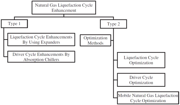
There are two types of natural gas liquefaction cycle enhancements described in this chapter as shown in Figure 1. The first type is modifying the liquefaction cycle by changing the cycle configuration by adding a new process/component or replacing the current process/component with the new process/component. This type of enhancement will be discussed in Section “Energy consumption enhancement options by recovering process losses and waste heat” for both liquefaction cycle and driver cycle enhancements. Enhancement of the liquefaction cycle by using expanders and enhancement of driver cycles by using absorption chillers are used as examples for this enhancement type.
Figure 1 Two types of natural gas liquefaction cycle enhancements
The second type of enhancement is optimization of the current cycle processes/components. Here optimization refers to the procedure of setting process design variables in such a way that all the design criteria are met and the energy consumption is minimized. An optimal natural gas liquefaction cycle should use lower energy consumption than an unoptimized natural gas liquefaction cycle. A brief overview of the optimization methods with an example explaining Genetic Algorithm (GA) are presented in Section “Brief introduction to optimization”. In Sections “Liquefaction cycle optimization” and “Driver cycle optimization”, the application of optimization in design enhancements of the liquefaction cycles and compressor driver cycles are discussed. The challenges in optimizing mobile natural gas liquefaction cycles are described in Section “Mobile LNG plants optimal design challenges”.
Energy consumption enhancement options by recovering process losses and waste heat
The first step in enhancing natural gas liquefaction cycles is allocating the location where unnecessary entropy is generated. In the liquefaction cycle, the entropy is generated in heat exchangers, expansion valves, and compressors. In the driver cycles, the entropy is generated in the compressor, combustion chamber, and turbine. Moreover, the exhaust of the gas turbine generates significant amounts of entropy due to its temperature difference with the ambient temperature. Here in this section, as a case of enhancing the liquefaction cycle, the effect of reducing the entropy generation by replacing expansion valves with expanders is considered. For the driver cycle enhancement case, the effect of employing absorption chillers powered by the gas turbine waste heat is considered.
Expanders
The liquefaction cycle efficiency could be improved by replacing expansion valves with expanders. Here the expanders refer to any mechanical device that converts the pressure exergy (maximum recoverable work by reducing the refrigerant pressure) of a fluid to work by reducing its pressure. The reason for enhancement is that the fluid undergoes isenthalpic expansion process through the expansion valve while it ideally undergoes isentropic expansion process through the expander. The entropy increases during the isenthalpic expansion process is expressed in Equation 1 based on the Maxwell relation.
where \( \style{font-size:22px}{h,\;T,\;s,\;v} \), and \( \style{font-size:22px}P \) are specific enthalpy, temperature, specific entropy, specific volume, and pressure. This means that the enthalpy of the fluid after expansion process will be higher in the case of isenthalpic expansion process than that of isentropic expansion process. Hence in the case of expanding the refrigerant using expansion valves, the vapor quality of the refrigerant will be higher than that using the expander. This will result in lower cooling capacity per unit mass of the refrigerant. Meanwhile compression work per unit mass of the refrigerant stays constant for both cases. Therefore, replacing expansion valves with expanders will increase the liquefaction cycle energy efficiency.
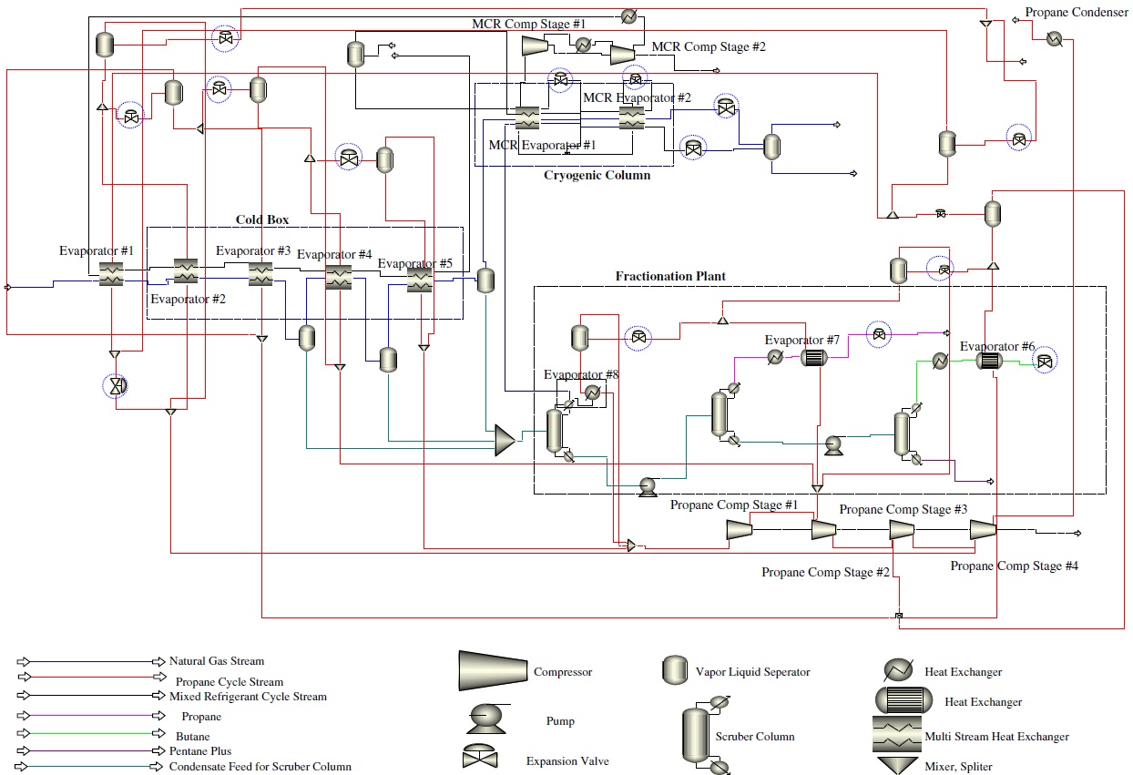
There are three types of expanders: liquid turbines, two-phase expanders, and gas expanders. Liquid turbines or hydraulic turbines are a well-established technology. They are available with efficiencies over 90 %. In order to apply them to a refrigeration cycle, the refrigerant should be subcooled before entering the turbine. This should be done to prevent evaporation of the refrigerant inside of the liquid turbine. Two-phase expanders are under development with current efficiencies in the vicinity of 80 % and can easily replace expansion valves used in vapor compression cycles. For expanding gases, gas expanders could be used instead of expansion valves. Gas expanders or gas turbines are a readily available technology and typically exist with efficiencies greater than 80 %. Mortazavi et al. (2011) studied the effect of replacing expansion valves with expanders on the performance of propane precooled mixed component refrigerant (MCR) liquefaction cycle. The schematic diagram of this cycle is shown in Figure 2. In the figure, the expansion processes that potentially can be recovered are marked with blue dashed circles.
Figure 2 Schematic diagram of the propane precooled MCR liquefaction cycle with the points that have a potential of recovering expansion losses shown by dashed circles
The effect of replacing expansion valves used in the MCR and propane cycles and the LNG expansion process with expanders was investigated by Mortazavi et al. (2011). In their study, for replacing expansion valves used in the MCR cycle and the LNG expansion process, only two-phase expanders were considered. However, in the propane cycle both two-phase expanders and liquid turbines used for expansion of the liquid propane and the gas expander used for expansion of gaseous propane were considered for replacing the expansion valves. In their study the following four different enhancement options were modeled:
Option 1. Enhancing the liquefaction cycle by replacing the LNG expansion valves by two-phase expanders. In Figure 2, the LNG expansion valves are located after the cryogenic column;
Option 2. Improving the liquefaction cycle by replacing the expansion valves of the MCR cycle with two-phase expanders in addition to the enhancement of Option 1;
Option 3. Improving the plant by replacing all the expansion valves with two-phase expanders for expanding liquid, and with gas expanders for expanding gas;
Option 4. Enhancing the cycle by replacing the propane cycle expansion valves with liquid turbines for expansion of liquid propane and replacing the rest of the expansion valves with two- phase expanders and gas expanders.
It should be noted that when replacing the propane cycle expansion valves with liquid turbines the refrigerant (propane) should be subcooled before the expansion process to minimize the evaporation of the refrigerant inside of the turbine. Therefore, a slight change should be made to the propane cycle to subcool the refrigerant to near the saturation temperature corresponding to the expander outlet pressure. In the study, the isotropic efficiency of the gas expander, liquid turbines, and two-phase expanders were assumed to be 0.86, 0.85, and 0.85, respectively . The modeling results of these enhancement options are shown in Table 1.
Table 1. Modeling Results of APCI Enhanced Cycles
Cycle Option
Base Cycle
Option 1
Option 2
Option 3
Option 4
Propane cycle compressor power [MW]
43.651
43.651
42.953
42.774
42.143
MCR cycle compressor power [MW]
66.534
66.534
65.375
65.375
65.368
Propane cycle cooling capacity [MW]
115.469
115.469
113.939
113.937
113.962
MCR cycle cooling capacity [MW]
67.635
67.635
67.634
67.635
67.631
LNG vapor fraction after the expander
0.0142
0.0006
0.0006
0.0006
0.0006
Total power consumption [MW]
110.185
110.185
108.324
108.148
107.506
Flash gases after LNG expander [kg/s]
1.28
0.05
0.05
0.05
0.05
Energy consumption per unit mass of LNG [MJ/kg]
1.115
1.101
1.083
1.081
1.074
Recovered power from expanders [MW]
–
0.648
2.528
3.296
3.821
LNG production [kg/s]
98.83
100.06
100.06
100.06
100.06
As can be seen from Table 1, the liquefaction cycle enhanced by Option 4 is the most efficient cycle among the cycles investigated. Based on their results, its total power consumption, flash gases after the LNG expander, and energy consumed per unit mass of LNG are lower than those of the base cycle approximately by 2.43 %, 96.09 % and 3.68 %, respectively. Moreover the expanders were expected to recover about 3.47 % of total consumed power. Based on their modeling, the LNG production was also higher than that of the APCI base cycle by 1.24 % from the same amount of feed gas.
They claimed, if the recovered power is deducted from the total power consumption, the energy consumed per unit mass of LNG could be reduced by 7.07 %. Since replacing expansion valves with expanders mainly utilizes the pressure exergy of the refrigerant, which is not significant, the efficiency enhancements were small. Although the enhancements were not considerable from a percentage point of view, if it is seen from an energy perspective it will lead to considerable savings and recovered power due to the scale of the plant.
Absorption chiller
One of the avoidable entropy generation sources in the natural gas liquefaction plant is waste heat produced from driver cycles. A waste heat source is defined as any hot exhaust gases or other streams that are cooled by rejecting heat to the ambient. The amount of avoidable entropy is proportional to the temperature difference between these streams and ambient temperature. The main sources of waste heat typically available at LNG plants are:
Gas turbine exhaust gases;
Flared gases;
Boiler exhaust gases.
Based on the waste heat temperature, the amount of waste heat, and utility requirement, such waste heat could be utilized for water desalination, air conditioning, refrigeration, gas turbine inlet cooling, heating, steam generation, and power generation. As an example case, the use of waste heat in enhancing the energy efficiency of a propane precooled MCR natural gas liquefaction cycle is considered. This study is taken from Mortazavi et al. (2010). In their study the waste heat from the gas turbine that drove the propane and MCR compressors was utilized to generate cooling from absorption chillers. Absorption chillers are the machines that convert heat to the refrigeration effect. There are a number of absorption chiller technologies with different applications. One of the measures used to evaluate absorption chiller performance is coefficient of performance (\( \style{font-size:22px}{COP} \)). \( \style{font-size:22px}{COP} \) is defined as the amount of cooling provided by the absorption chiller divided by the amount of energy consumed by the absorption chiller. Most absorption chillers use either water/lithium-bromide or ammonia/water as their working fluid pair. In working fluid nomenclature the first part represents the refrigerant and the second part represents the absorbent fluid. Water/lithium-bromide absorption chillers tend to have higher \( \style{font-size:22px}{COPs} \) compared to ammonia/water chillers. Meanwhile, the water/lithium-bromide absorption chillers evaporator cannot be below about 2 °C due to water freezing; moreover there is crystallization issue if they are operated with high absorber temperature. On the other hand, ammonia/water absorption chillers evaporator temperature can be lower than -30 °C. Conventional absorption chillers can be single or double-effect. Single-effect absorption chillers are less complex by having less number of components and requiring lower temperature waste heat; however their \( \style{font-size:22px}{COPs} \) are lower than those of double-effect chillers. For more information regarding the absorption chillers please refer to Herold et al. (1996).
To quantify the amount of available waste heat from the gas turbine, gas turbine exhaust tem-perature and mass flow rate should be assessed. In the Mortazavi et al. (2010) study such information was derived by modeling the gas turbine. The comparison of the gas turbine simulation results with vendors’ data at ISO condition, which is 15 °C and 1 atm inlet pressure, is shown in Table 2.
Table 2. Comparison of Gas Turbine Modeling Results with Vendors’ Data at ISO Condition
Parameter
ISO Rated Power [MW]
Efficiency [%]
Exhaust Temperature [°C]
Actual gas turbine
130.100
34.6
540.0
ASPEN model
130.103
35.0
540.4
Discrepancy
+0.003 (0.0 %)
+0.4 (1.16 %)
+0.4
In the study a double-effect design was selected based on the gas turbine exhaust temperature and the minimum temperature that the exhaust can be cooled. It should be noted that lowering the exhaust temperature below 180 °C increases the chance of corrosion due to condensation. They selected water/lithium-bromide as a refrigerant/absorbent pair due to its superior \( \style{font-size:22px}{COP} \) compared to ammonia/water. In their investigation they assumed that the plant is located on the Persian Gulf coast with 45°C ambient temperature and 35 °C seawater temperature. Based on these ambient conditions they modeled a double-effect water/lithium-bromide chiller for two different evaporating temperatures corresponding to the two highest temperature stages of the propane cycle. Their modeling results are shown in Table 3. The\( \style{font-size:22px}{COP} \) values were used to estimate the amount of waste heat that is needed to produce the amount of cooling required for different enhancement options.
Table 3. Modeling Results of Absorption Cycle
Evaporating Temperature
COP
9 °C
1.284
22 °C
1.489
For a fixed production capacity, the energy consumption of a liquefaction cycle could be reduced by either reducing the compressor power demand or increasing the gas turbine power generation efficiency. The absorption chiller’s cooling can be used to reduce the compressor’s power demand. This reduction can be done by lowering the propane cycle condenser temperature, replacing the propane evaporators by waste heat powered absorption chillers, and/or intercooling the compressor of the MCR cycle. Moreover, the absorption chiller’s cooling can be used to increase gas turbine power generation efficiency by cooling the inlet air of the gas turbine.
Mortazavi et al. (2010) developed an integrated gas turbine and liquefaction cycle model to investigate the available amount of waste heat for different enhancement options. In their integrated model, their gas turbine model was scaled to satisfy the liquefaction cycle power demand at 45 °C ambient temperature under its full load condition. Scaling the gas turbine is not an unreasonable assumption due to the fact that some gas turbine manufactures scale their gas turbine design to meet for different demands. Eight enhancement options of waste heat utilization using absorption chillers were considered, as summarized in Table 4.
Table 4. Different Waste Heat Utilization Options
Option
Description
1
Replacing 22 °C propane cycle evaporators with absorption chillers
2
Replacing 22 °C propane cycle evaporators and cooling the inlet of gas turbine with absorption chillers
3
Replacing 22 °C and 9 °C propane cycle evaporators with absorption chillers
4
Replacing 22 °C and 9 °C propane cycle evaporators and cooling the inlet of gas turbine with absorption chillers
5
Replacing 22 °C and 9 °C evaporators and cooling the condenser of propane cycle at 27 °C with absorption chillers
6
Replacing 22 °C and 9 °C evaporators and cooling the condenser of propane at 27 °C cycle and turbine inlet with absorption chillers
7
Replacing 22 °C and 9 °C evaporators and cooling the condenser of propane cycle at 14 °C with absorption chillers
8
Replacing 22 °C and 9 °C evaporators and cooling the condenser of propane at 14 °C cycle and intercooling the compressor of mixed refrigerant cycle with absorption chillers)
To account for part load effects they considered two cases for each enhancement option. The first case, which was referred to as an unscaled case, was based on the assumption that for each option the gas turbine would be the same size as that of the base cycle (cycle without enhancement). This assumption allowed them to observe some part load degradation effects. The second case, referred to as a scaled case, was based on the assumption that for each option a gas turbine is sized to provide the maximum liquefaction cycle power plant demand at its full load. In their modeling they assumed the gas turbine exhaust gas could be cooled down to 200 °C. Their simulated enhancement option results are shown in Table 5.
Table 5. Enhancement Results of Different Waste Heat Utilization Options
Gas Turbine Sizing
Scaled Turbine Size Case
Unscaled Turbine Size Case
Option
Compressor Power [MW]
Power Reduction [MW]
Required Amount of Waste Heat [MW]
Fraction of Available Amount of Waste Heat [%]
Fuel Consumption [MW] (% saving)
Required Amount of Waste Heat [MW]
Fraction of Available Amount of Waste Heat [%]
Fuel Consumption [MW] (% saving)
Base cycle
110.185
–
–
–
329.448
–
–
329.448
Option 1
107.510
2.675 (2.43 %)
8.865
5.948
321.444 (2.43)
8.865
5.958
322.754 (2.03)
Option 2
107.510
2.675 (2.43 %)
12.572
8.985
314.002 (4.69)
12.913
9.341
318.175 (3.42)
Option 3
100.334
9.851 (8.94 %)
34.998
25.162
299.999 (8.94)
34.998
25.311
304.859 (7.46)
Option 4
100.334
9.851 (8.94 %)
41.579
33.537
287.624(12.70)
43.112
36.306
296.482 (10.01)
Option 5
94.043
16.142 (14.65 %)
98.306
75.408
281.186 (14.65)
98.306
76.133
289.482 (12.21)
Option 6
94.043
16.142 (14.65 %)
104.474
89.899
269.598 (18.17)
106.420
96.977
281.006 (14.70)
Option 7
88.420
23.489 (21.32 %)
105.553
86.112
264.378 (19.75)
105.553
87.227
275.340 (16.42)
Option 8
86.696
23.489 (21.32 %)
116.391
96.844
259.217 (21.32)
116.391
98.195
271.086 (17.72)
Открыть таблицу в новом окне
As Table 5 shows, the options are placed based on their energy efficiency enhancement order, where Option 8 has the highest amount of enhancement. Based on their results, by implementing Option 8 the compressor power demand and hence gas turbine fuel consumption could be reduced by 21.3 %. Within all the options the scaled gas turbine cases have lower fuel consumption than those of the unscaled cases. This difference indicates that the efficiency of the scaled case is higher than the unscaled case for the same option. This difference is due to the fact that in the unscaled case the gas turbine is operated at part load running condition, whereas in the scaled case the gas turbine is operated in full load. Meanwhile the gas turbine firing temperature in part load conditions are lower than the full load condition, which leads to lower efficiency of the gas turbine. Based on Table 5, the better the option, the more amount of waste heat is required to operate the absorption chillers, which means less entropy generation.
Brief introduction to optimization
Design of a system involves selecting variables that meet system requirements that are defined beforehand by a customer. For example, a heat exchanger designer needs to know the required heating load and other product requirements specified by the customer. Then the designer would select design variables such as the heat exchanger material, dimensions, and so on that meet the heat exchanger requirements. Several heat exchanger designs could be developed that meet the same heat load requirements. However, the heat exchanger’s performance and cost depend on the selected variables.
The optimal design represents the design that has the most desired objectives, such as minimum cost or highest performance.
In the conventional design approach, the process of selecting design variables is based on a designer’s intuition and experience. A designer could achieve optimal design with the conventional design approach when designing simple products, which have only a limited number of design variables. On the other hand, it is difficult and could be impossible to achieve optimal design with the conventional design approach when designing complex systems with many variables.
The process of finding the optimal design is called optimization. Optimization uses mathematical techniques to achieve the optimum design. In the optimization formulation, there is an objective function whose value should be optimized. Moreover, there might be some constraints that should be satisfied by the optimum design. In an optimization procedure, any point that satisfies the constraints is called a feasible point. The variables that are varied during an optimization procedure are called design variables. The variables that are assumed to be fixed during an optimization procedure are called design parameters. It should be noted that an optimization problem can have multiple objective functions. This kind of optimization is called a multiobjective optimization.
There are two types of optimization problems, deterministic (conventional) and stochastic. In the deterministic optimization it is assumed that there is no uncertainty in the design variables and parameters. However, in the stochastic optimization problems the uncertainties in the design variables and parameters are considered. One class of stochastic optimization problems is robust optimization. In robust optimization the solutions should be feasible for all variations of the uncertain variables and parameters. Mathematically the deterministic optimization problems are stated as follows:
where \( \style{font-size:22px}{f,\;g_i} \), and \( \style{font-size:22px}{h_j} \) are called objective function, inequality constraint, and equality constraint, respectively. \( \style{font-size:22px}x \) is vector of design variables, and p is vector of design parameters. In deterministic optimization, design parameters are fixed but design variables are varied. An overview of conventional optimization methods is presented in Section “Conventional optimization methods”. Section “Robust optimization methods” provides a brief overview of robust optimization.
Conventional optimization methods
Generally optimization methods can be classified into general methods and methods tailored for a specific class of problems. Specific methods such as linear programming and quadratic programming are more efficient than the general methods in solving the problems because they are tailored for it. However, they are not applicable to general problems. General methods can be divided to local optimization methods and global optimization methods. Except for specific problems, local optimi-zation methods only provide results that are locally optimal. However, their computational cost is lower than those of global search methods. Newton method and sequential quadratic programming are examples of local optimization methods. Global optimization methods are heuristic-based methods.
This means that there is no guarantee for their result to be globally optimal. Genetic algorithm (GA) and simulated annealing are examples of methods that do not have any restriction in the type of functions that are used in stating the objective and constraint functions. The GA optimization method will be explained briefly in the next section because it was used in the LNG plant refrigerant and driver optimization sections. Interested readers are referred to optimization books such as Bazaraa et al. (1993), Arora (2004), or Gen and Cheng (2007).
Genetic algorithm
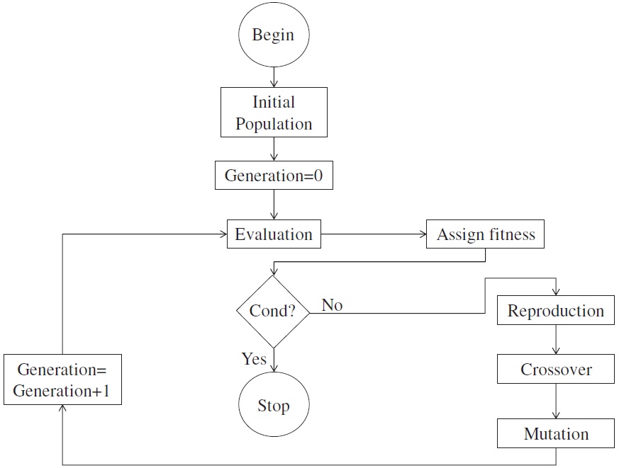
Genetic algorithm (GA) is a class of heuristic optimization methods. GA mimics the process of natural evolution by modifying a population of individual solutions. Design points, x’s, are represented by chromosomes. The method randomly selects individuals from the current population to be parents and uses them to produce the children for the next generation. Over consecutive generations, the population approaches an optimal solution because “good” parents produce “good” children. The “bad” points are eliminated from the generation. GA can be applied to solve a variety of optimization problems in many applications that are not suited for conventional optimization methods, including problems in which the objective function is discontinuous, nondifferentiable, or nonlinear. GA has the potential to reach the global optimal solution if it does not stick at a local optimal solution. Since GA is a probabilistic approach, different solutions could be generated by different runs. Therefore, multiple runs are required to verify the optimal solution. A GA flowchart is shown in Figure 3. The steps involved in using GA are described in the following sections, using a simple refrigerant composition optimization problem detailed next.
Figure 3 Flowchart showing working principle of GA
Example of GA
Finding the optimal refrigerant composition is difficult without optimization. Suppose we would like to find the optimal refrigerant composition of mixture for a vapor compression cycle that has a given cooling load. The optimal refrigerant would require less compression power for the same cooling provided. The formulation of the optimization problem is as follows:
Objective function:
Minimize compressor power (\( \style{font-size:22px}{x_1,\;x_2,\;x_3,\;x_5,\;x_6} \)), where;
\( \style{font-size:22px}{x_1,\;x_2,\;x_3,\;x_4} \) are mass fractions of constituents;
\( \style{font-size:22px}{x_5} \) total refrigerant mass flow rate;
\( \style{font-size:22px}{x_5} \) and \( \style{font-size:22px}{x_6} \) were assumed to be limited by a 20 % range from the baseline values so that we have a limited design space.
Representing a solution
GA represents the variables as binary strings. In the example, we have five variables because \( \style{font-size:22px}{x_4} \) is not an independent variable. Each variable is coded in 4 bits. The more bits we have, the more precise the variables would be. Since we assumed 4 bits, each variable can have \( \style{font-size:22px}{2^4} \) possible values. One 20-bit string (or chromosome) that represents one solution is as follows:
For example, x6 is represented in this string as 0001, which represents a certain value for the refrigerant condensing pressure within the specified lower and upper limits. The same principle is true for the other variables. Thus, this chromosome represents a design that has a corresponding compressor power as well as values for meeting or violating the constraints. In the beginning of the GA, a population of chromosomes is randomly generated to be evaluated in the next steps. The number of the generated chromosomes can be taken to be 20 times the number of the decision variables.
Assigning a fitness to a solution
Once the initial population was generated, a fitness function is assigned to evaluate the “goodness” or “badness” of a solution or a chromosome. In a minimization problem, the good solution has small fitness function value and the bad solution has high fitness function value. The generated solutions are evaluated based on the objective function value and constraints violation. In our example, the objective function is the minimization of the compressor power and the constraints are the evaporator capacity and temperature. Following fitness assignment, the GA checks for termination conditions and, if not met, a new population is generated based on three genetic operators, which are the reproduction, crossover, and mutation operators.
Reproduction operator
The reproduction operator duplicates “good” solutions and eliminates “bad” solutions in the popu-lation. Different methods exist in the reproduction operator such as tournament selection or ranking selection. Tournament selection method, for example, compares two solutions and the best one survives in the mating pool. Ranking selection method lists the population based on individual solutions’ fitness values. As the GA runs, only “good” solutions survive in the population.
Crossover operator
The reproduction operator does not generate a new solution. It just duplicates “good” solutions and eliminates “bad” solutions. On the other hand, the crossover operator is used to generate new solutions. It selects two chromosomes, called parents (e.g., A and B in Figure 4), from the mating pool and exchanges bits at certain points to generate a new solution, which is called offspring (e.g., A1 and B1 in Figure 4). The “good” parents hopefully will produce “good” offspring.
Figure 4 Crossover operator. (Solution A and B are called parent solution while A1 and B1 are called offspring.)
Mutation operator
The mutation operator has the same objective as the crossover operatordto generate new solutions and possibly jump out from a local optimum. It works by exchanging a string in the mating pool from 0 to 1 or vice versa as shown in Figure 5.
Figure 5 Mutation operator. (Solution A1 is old solution and Solution A2 is the new solution.)
Stopping criteria
Different stopping criteria can be implemented in GA. Common stopping criteria are reaching the maximum number of generations or the change in the best solution in successive iteration is less than the prespecified value (convergence tolerance).
Robust optimization methods
One of the main challenges in engineering optimization is that the deterministic optimization algorithms do not account for the uncertainty involved in the design process. Neglecting the uncertainties (in design parameters and variable) could result in designs that are infeasible or have a poor performance. The uncertainty in design variables might be reducible by using more precise manufacturing techniques, which would increase production cost. However, there are uncontrollable parameters such as weather conditions, energy price, and market demand, whose uncertainties are not reducible. Therefore, deterministic optimization might not be the best optimization technique for many of the real world engineering problems. The goal of robust optimization algorithms is finding an optimal solution that is insensitive to design variables and parameter uncertainty. This design is called a robust design. There are two types of robustness: objective robustness and feasibility robustness. A design x is said to be objectively robust if the objective variation remains in the specific range for all realizations of the design variables and parameters in their uncertainty range. Here the robustness formulation is developed for problems in which the uncertainty is in the form of a symmetric interval with the nominal point as its center. Mathematically objective robustness can be stated as
where \( \style{font-size:22px}{\Delta f\ast} \) is the acceptable variation of the objective function. \( \style{font-size:22px}{\Delta\overline x} \) and \( \style{font-size:22px}{\Delta\overline p} \) are the design variables and parameters uncertainty range and they are nonnegative vectors.
For the problem where the objective robustness is based on the degradation of the objective function Equation 3 becomes (Mortazavi et al., 2012):
In Equation 4 it is permissible if the variation of the uncertain design variables and parameters reduce the objective function value. However, if it is increasing the objective function value it should be a less than acceptable deviation of the objective function.
A design X is defined to be robust feasible if it stays feasible for all the realizations of the design variables and parameters in their uncertainty range. Mathematically it is shown as
Note that the equality constraints do not exist in robust optimization. This is due to the fact that it is not possible to maintain an equality constraint when there is a variation (due to uncertainty) in design variables and parameters.
Up to now all the natural gas liquefaction cycle optimizations were conducted without implementing the robust optimization techniques. Therefore their results might become infeasible in the real world operating conditions. In the real world application, designers are using safety factors to account for the uncertainties. Although this approach might lead to a robust design it usually does not lead to an optimum robust solution. It is proposed to use robust optimization techniques to find the realistic enhancement design option for the liquefaction cycle. This will increase the applicability of these enhancement options to the real-world LNG plants.
Liquefaction cycle optimization
As explained earlier, the GA has the capability of optimizing a natural gas liquefaction cycle. Since among all available cycles, the APCI liquefaction cycle, developed by Air Products and Chemicals Inc., is the most predominant cycle in the LNG industry, it was selected to demonstrate the power of optimization using GA. The optimization approach followed here would be similar when it is applied to different liquefaction cycles optimization. More details on the liquefaction cycle optimization problem and a comparison between different optimization results obtained from different optimization methods can be found in Alabdulkarem et al. (2011).
Model development
The model of the APCI liquefaction cycle can be found in Mortazavi et al. (2010). The model was based on ASPEN Plus software v7.1 (2010), which is a robust steady-state process simulation software. ASPEN Plus has a built-in optimization tool. However, it does not have GA methods available and we were not able to link it with MatLab (2009), which has GA as well as different optimization tools. On the other hand, HYSYS v7.1 (2010), a steady state and transient process simulation software, does not have a GA either but we were able to link it with MatLab and utilize its optimization capabilities. Therefore, a model was developed using HYSYS for the APCI liquefaction cycle with the same inputs and assumptions used in the ASPEN Plus model. The inputs and assumptions used in the two models are essentially identical
Gas sweetening units were not modeled for simplification purposes and the feed gas was assumed to be after the sweetening units with the composition shown in Table 6.
Table 6. Gas Composition after Gas Sweetening
Component
Mole Fraction (%)
Nitrogen
0.100
Carbon Dioxide
0.005
Methane
85.995
Ethane
7.500
Propane
3.500
i-Butane
1.000
n-Butane
1.000
i-Pentane
0.300
n-Pentane
0.200
Hexane Plus
0.400
Total
100
The two sections of the spiral-wound heat exchanger (SPWH) were modeled using the segmented UA method. Using the segmented UA method means applying the UA method on several intervals inside the heat exchanger so that the cooling curve inside the SWHX is calculated more accurately. The first section of the SPWH has 53 segments and the second section has 38 segments. Simulation results from models in HYSYS and ASPEN Plus are compared in Table 7.
Table 7. Simulation Results of APCI Base Cycle Model in ASPEN Plus and HYSYS
Model
ASPEN Plus
HYSYS
Discrepancy (%)
Propane compressor power (MW)
43.651
43.698
-0.1
Mixed refrigerant compressor power (MW)
66.534
66.48
0.08
Propane cycle cooling capacity (MW)
115.469
115.733
-0.22
Mixed refrigerant cycle cooling capacity (MW)
67.635
67.508
0.18
Propane cycle coefficient of performance
2.645
2.648
-0.13
LNG vapor fraction after expansion valve (%)
1.4
1.43
-2.14
LNG production (kg/s)
98.83
98.89
-0.06
LPG (propane, butane, pentane, and heavier hydrocarbons) (kg/s)
11
10.97
0.27
Flash gas flow rate after LNG expansion valve (kg/s)
1.28
1.24
3.13
It can be seen that there is a good agreement between the two software models. The reason for the discrepancies in some parameters is due to the fact that the binary coefficients of the equation of state used in HYSYS and ASPEN Plus are slightly different from each other. The schematic of the APCI liquefaction cycle modeled in HYSYS is shown in Figure 6.
Figure 6 APCI liquefaction cycle’s HYSYS model
There is a break point in the process flow sheet, which is required for HYSYS and ASPEN Plus model convergence. However, inside the MatLab code the two sides of the break point are set to be identical to each other.
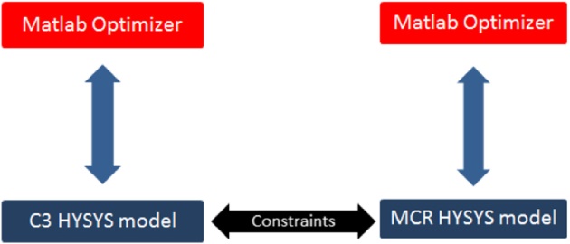
Optimization approach
Since there are many variables involved in designing the APCI liquefaction cycle, the optimization problem is computationally very expensive. Thus, the optimization was carried out in two stages as shown in Figure 7. First, the MCR cycle was optimized, and then the propane cycle was optimized. The only effect of separating the two cycles is that the propane cycle precools the MCR cycle. This precooling load changes with refrigerant mixture composition, temperature, pressure, and mass flow rate. This effect was considered as optimization constraints. MatLab has a powerful optimization tool. It has different optimization methods such as gradient-based and GA. To verify the results of the optimization, different optimization methods (e.g., gradient-based or pattern search; Arora, 2004) from MatLab as well as optimization tools from the HYSYS and ASPEN were used. Results show that the optimum results (i.e., minimum power consumption) were found with the GA method. For instance, the pattern search optimization method resulted in a 7.16 % saving in MCR power consumption whereas the GA resulted in a 13.28 % saving in MCR power consumption for an identical optimization problem.
Different optimization methods lead to different results (e.g., different refrigerant composition mixtures). A comparison of different optimization methods to find refrigerant composition mixtures was conducted by Alabdulkarem et al. (2011). The number of design variables for the MCR cycle is eight, compared with 14 for the propane cycle. Each cycle takes between 16 and 24 hours to solve with a desktop computer having an Intel Core 2 Duo processor (2.83 GHz) CPU with 2 GB of RAM. Typical GA tuning parameters used in the optimization are listed in Table 8.
Table 8. Typical GA Tuning Parameters
Tuning Parameters
Value
Population size
20 × number of design variables
Reproduction count
50 % of the population size
Maximum number of generations
100
Crossover fraction
0.8
Selection method
Tournament
Tournament size
8
Fitness scaling method
Top
Number of crossover points
1
Mutation method
Adaptive feasible
The objective function of the MCR cycle optimization and propane cycle optimization is to reduce the total power consumption of the APCI liquefaction cycle. The power consumption comes from the compressors and seawater pumps, as calculated by HYSYS software. The model in HYSYS is treated as a black box in this optimization study. The variables of the MCR optimization are listed in Table 9.
Table 9. List of MCR Cycle Optimization Variables
Variable
Baseline Value
Refrigerant mass flow rate (kg/s), \( \style{font-size:22px}{\dot m} \)
270
Nitrogen refrigerant mass fraction, \( \style{font-size:22px}{X_{N2}} \)
0.0971
Methane refrigerant mass fraction, \( \style{font-size:22px}{X_{C1}} \)
0.2225
Ethane refrigerant mass fraction, \( \style{font-size:22px}{X_{C2}} \)
0.5445
Propane refrigerant mass fraction, \( \style{font-size:22px}{X_{C3}} \)
The range of the optimization variables is taken to be ±20 % of the baseline values. The MCR optimization’s seven constraints with limits taken from the baseline model are:
Temperature of the LNG < -160 °C;
LNG mass flow rate = 98.89 kg/s;
Precooling load of the propane cycle < 88.22 MW;
Two compressors with inlet vapor quality > 0.99;
Two heat exchangers with pinch temperatures > 3 °K.
The propane cycle optimization variables are listed in Table 10. The range of the optimization variables is also taken to be ±20 % of the baseline values.
Table 10. List of Propane Cycle Optimization Variables
22 °C Heat exchanger pressure (kPa), \( \style{font-size:22px}{x_7} \)
882
Refrigerant mass splitter to the -19 °C \( \style{font-size:22px}{HX} \) split ratio, \( \style{font-size:22px}{x_8} \)
0.465
Refrigerant mass splitter to the -5 °C \( \style{font-size:22px}{HX} \) split ratio, \( \style{font-size:22px}{x_9} \)
0.758
Refrigerant mass splitter to the 9 °C \( \style{font-size:22px}{HX} \) split ratio, \( \style{font-size:22px}{x_10} \)
0.143
Refrigerant mass splitter to the 16 °C \( \style{font-size:22px}{HX} \) split ratio, \( \style{font-size:22px}{x_11} \)
0.886
Refrigerant mass splitter to the 22 °C \( \style{font-size:22px}{HX} \) split ratio, \( \style{font-size:22px}{x_12} \)
0.705
Refrigerant mass splitter to liquefy the propane produced, \( \style{font-size:22px}{x_13} \)
0.909
Refrigerant mass splitter to liquefy the butane produced, \( \style{font-size:22px}{x_14} \)
0.938
Changing an intermediate compressor outlet pressure is equivalent to changing a corresponding evaporation temperature because each heat exchanger/evaporator is connected to a compressor outlet. The propane cycle optimization’s 17 constraints with limits taken from the baseline model are:
Three LPG produced vapor quality < 0.01;
Propane fuel production = 2.95 kg/s;
Pentane plus fuel production = 5.1 kg/s;
Butane fuel production = 2.92 kg/s;
Condensing load of the fractionation unit = 5.07 MW;
Four compressors with inlet vapor quality > 0.99;
Six heat exchangers with pinch temperatures > 3 °K.
Optimization results
The optimization results of the APCI natural gas liquefaction cycle are described in Section “MCR cycle optimization” for the MCR cycle optimization and Section “Propane cycle optimization” for the propane cycle optimization.
MCR cycle optimization
The optimized MCR cycle has a power consumption of 63.63 MW, which is 4.48 % less than the baseline power consumption. The optimized MCR cycle has lower refrigerant mass flow rate and lower overall compression ratio than those of the baseline cycle as shown in Table 11.
Table 11. MCR Cycle Optimization Results
Cycle
Variables
Objective Function
\( \style{font-size:22px}{\dot m} \) (kg/s)
\( \style{font-size:22px}{X_{N2}} \)
\( \style{font-size:22px}{X_{N2}} \)
\( \style{font-size:22px}{X_{C2}} \)
\( \style{font-size:22px}{X_{C2}} \)
\( \style{font-size:22px}{X_{C2}} \)
\( \style{font-size:22px}{P_H} \)
\( \style{font-size:22px}{P_H} \)
Min. Power Cons. (MW)
Baseline
270
0.0971
0.2225
0.5445
0.1359
2300
4000
420
66.62
Optimized
267
0.1027
0.218
0.5306
0.1487
2346
4137
451
63.63
(Variable definitions are given in Table 10)
Nitrogen and propane mass fraction increased while the methane and ethane decreased. Since nitrogen has the lowest boiling temperature among the constituents, it lowers the lowest refrigeration temperature. On the other hand, propane has the highest boiling temperature, which increases the refrigeration capacity of the refrigerant. A plot of the cooling curves for the optimized and baseline MCR cycles is shown in Figure 8.
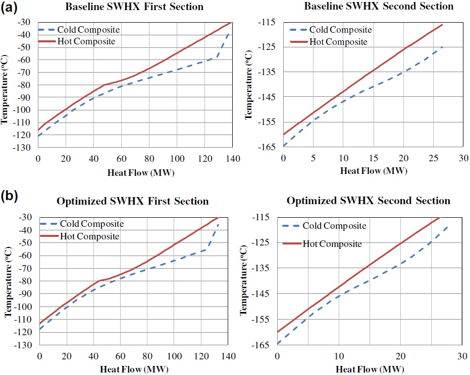
Figure 8 Cooling curves in SWHX of the (a) baseline and (b) optimized MCR cycles. The cooling curves are closer to the heating curves in the optimized cycle than the baseline cycle at equivalent pinch temperature of 3 °K
The SWHX has two sections with log mean temperature difference (LMTD) for the optimized cycle of 5.24 °C and 4.91 °C, whereas the LMTDs of the baseline cycle are 7.12 °C and 5.17 °C. Figure 8 and the LMTD values show that the cold curve in the optimized cycle is closer to the hot curve than the baseline cycle, which means more efficient heat transfer or less entropy gen-eration in the heat exchanger.
Propane cycle optimization
The optimized propane cycle has a power consumption of 37.15 MW, which is 15.98 % less than the baseline power consumption. The optimized propane cycle has a higher refrigerant mass flow rate, maximum subcooling, and slightly lower overall compression ratio than those of the baseline cycle as shown in Table 12.
Table 12. Propane Cycle Optimization Results
Cycle
Variables
Objective Function
\( \style{font-size:22px}{\dot m} \) (kg/s)
\( \style{font-size:22px}{T_c} \) (°C)
Pressures (kPa)
\( \style{font-size:22px}{x_1} \)
\( \style{font-size:22px}{x_2} \)
\( \style{font-size:22px}{x_3} \)
\( \style{font-size:22px}{x_4} \)
\( \style{font-size:22px}{x_5} \)
\( \style{font-size:22px}{x_6} \)
\( \style{font-size:22px}{x_7} \)
Baseline
447
43
253
406
618
882
1,540
Optimized
465
40
240
406
758
847
1,433
Cycle
Variables
Power Consumption (MW)
Split Ratios
\( \style{font-size:22px}{x_8} \)
\( \style{font-size:22px}{x_9} \)
\( \style{font-size:22px}{x_{10}} \)
\( \style{font-size:22px}{x_{11}} \)
\( \style{font-size:22px}{x_{12}} \)
\( \style{font-size:22px}{x_{13}} \)
\( \style{font-size:22px}{x_{14}} \)
Baseline
0.465
0.758
0.143
0.886
0.705
0.909
0.938
44.22
Optimized
0.449
0.7
0.143
0.905
0.705
0.911
0.902
37.15
(Variable definitions are given in Table 10)
Split ratios, \( \style{font-size:22px}{x_8} \) and \( \style{font-size:22px}{x_9} \), are reduced so that an optimized amount of refrigerant is provided to low temperature heat exchangers at -19 °C and -33 °C, respectively, which has low expansion pressure that requires more compression power. The other split ratios, \( \style{font-size:22px}{x_{11},\;x_{13}} \), and \( \style{font-size:22px}{x_{14}} \), were adjusted by the optimizer to meet the change in the total mass flow rate. In order to know how much power savings were obtained due to lower condensing temperature, 40 °C was applied on the baseline model, which resulted in 0.817 MW power reductions from the total baseline cycle power consumption. Therefore, the optimized cycle power savings is due mainly to the optimized mass distributions and pressure levels.
Second law efficiency
The Second Law efficiency, Equation 7, is used to compare a thermodynamic cycle and an ideal reversible cycle. The minimum power to liquefy the natural gas (NG) to LNG and LPG is from the ideal reversible cycle using exergy difference, which is calculated by Equations 8 and 9.
where \( \style{font-size:22px}{\dot W} \) is the power, \( \style{font-size:22px}{\dot m} \) is the mass flow rate, ex is the exergy, h is the enthalpy, \( \style{font-size:22px}{T_0} \) is the ambient temperature, and s is the entropy.
The minimum reversible compressors power required for LNG and LPG production was calculated from Equation 8 to be 50.36 MW. The total power consumption of the baseline cycle, as well as that of the optimized cycle, was calculated by the model in HYSYS to be 110.84 MW and 100.78 MW, respectively. This resulted in a Second Law efficiency of 45.43 % for the baseline cycle and 49.97 % for the optimized cycle. The baseline natural gas liquefaction cycles model consumes 5.66 kWh energy per kmol of LNG produced whereas the optimized plant consumes 5.14 kWh energy per kmol of LNG produced.
Effect of pinch temperature
APCI liquefaction cycle uses SWHX, which is a proprietary heat exchanger developed by Linde Inc. This expensive heat exchanger is used in the cryogenic column and it has a low pinch temperature with a range as low as 3 °K. The other type of less expensive heat exchanger that is used for liquefying natural gas is a plate-fin heat exchanger. The effect of pinch temperature on the liquefaction cycle power consumption was investigated as shown in Table 13.
Table 13. Liquefaction Cycle Optimization Results with Different Pinch Temperatures
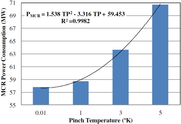
The optimizer, coupled by HYSYS, was run with four pinch temperatures: 0.01, 1, 3, and 5 °K. Different pinch temperatures represent the performance of different heat exchangers. Lowest pinch temperature (0.01 °K) represents extremely large, efficient, and high UA value heat exchangers as an ideal case. As shown in Figure 9, the savings in power consumption increases with the decrease in the pinch temperature.
Figure 9 Optimized MCR power consumption at different heat exchanger pinch temperatures
These savings can be translated to operating cost and then compared with initial cost for the economic evaluation of different s selections. Equation 10 fits the resulting optimized MCR power for different pinch temperatures.
where \( \style{font-size:22px}{P_{MCR}} \) is optimized MCR power consumption, MW; and \( \style{font-size:22px}{TP} \) is pinch temperature, °K.
Driver cycle optimization
The three components that have the most impact on the efficiency of a natural gas liquefaction cycle are heat exchangers, compressors, and compressor drivers. Most of the liquefaction plant energy consumption is due to the compressor drivers. In most cases the chemical energy of the fuel is converted to mechanical work to drive the compressors directly or to drive the electric motor driving the compressors. Gas turbines and steam cycles are conventionally used as drivers. The new plants are using mostly gas turbines as their drivers. However, the efficiencies of the gas turbines are below 50 %. Gas turbine efficiency value degrades if the gas turbine is operated below its nominal capacity. The efficiency of the combined cycles can reach 60 %.
In selecting the best option the economic aspects should also be considered. In optimization of the driver the main objectives are minimizing the annual energy consumption of the drivers or maximizing the annual production or profit. The typical constraints that should be met are the compressor power and the availability and reliability of the plant. Either the conventional optimization or stochastic optimization methods can be used for optimizing the driver cycles. However, if the conventional optimization is used, the nominal point should account for the typical worst scenario. Moreover, to cover the annual operation of the plant it is suggested dividing the year into several periods (bean) and setting the parameters as typical worst scenario for that period.
As a demonstration, a simple optimization driver problem is formulated. In this example the task is maximizing the profit for the plant where the compressors are electrically driven and the electricity is generated on site. There are “k” electrical power generator options. The goal is to select the best combination of these generators, their monthly operation schedule, and LNG monthly volumetric production.
\( \style{font-size:22px}{C_{m,LNG}} \): Volumetric price of LNG in month m;
\( \style{font-size:22px}{C_{m,NG}} \): Volumetric price of natural gas in month m;
\( \style{font-size:22px}{C_{m,\;operation}} \): Adjusted operational cost (including the capital cost ) except fuel cost of drivers;
\( \style{font-size:22px}{C_{m,\;other}} \): Adjusted operational cost of the liquefaction plant excluding the drivers;
\( \style{font-size:22px}{d_m} \): Total operation time in month m in hours;
\( \style{font-size:22px}{G_{j,Ava}} \): Adjusted availability of generator driver type \( \style{font-size:22px}j \) in hours per month;
\( \style{font-size:22px}{G_{j,m,\cos t}} \): Adjusted operational cost of generator driver \( \style{font-size:22px}j \) in month m;
\( \style{font-size:22px}{G_{j,m,P}} \): Nominal capacity of generator driver \( \style{font-size:22px}j \) in month m;
\( \style{font-size:22px}{n_j} \): Number of power generator type \( \style{font-size:22px}j \);
\( \style{font-size:22px}{P_{GT,m}} \): Maximum power generation capacity in month m;
\( \style{font-size:22px}{P_{LNG,m}} \): Liquefaction power demand in month m;
\( \style{font-size:22px}{PL} \): Percentage of part load (ratio of driver output to the nominal output at that condition)
\( \style{font-size:22px}{v_{m,LNG}} \): LNG production in month m;
\( \style{font-size:22px}{v_{m,driver}} \): Total natural gas consumption of generator drivers in month m;
\( \style{font-size:22px}{v_{m,min,LNG}} \): Minimum LNG production capacity in month m;
\( \style{font-size:22px}{v_{m,max,LNG}} \): Maximum LNG production capacity in month m;
\( \style{font-size:22px}{h_{j,m}} \): Efficiency of the generator driver type \( \style{font-size:22px}j \) at \( \style{font-size:22px}{PL} \) % part load condition.
The goal in this optimization problem is finding the optimum values of \( \style{font-size:22px}{v_{m,LNG,\;nj}} \) and \( \style{font-size:22px}{PL} \). The objective function (Equation 11) calculates the annual plant profit. It is based on the monthly profit of the natural gas liquefaction cycle. The monthly profit is the value of the produced LNG minus the adjusted operational, raw material, and fuel cost. Constraint \( \style{font-size:22px}{g_1} \) (Equation 12) ensures that the maximum power generation capacity in month m is higher than the power demand in that month. The power demand in month m is assumed to be a function of LNG production in that month. Constraint \( \style{font-size:22px}{g_2} \) (Equation 13) ensures that there will be enough generation capacity in month m.In constraint\( \style{font-size:22px}{\;g_2,G_{j,Ava}} \) is the average period that driver \( \style{font-size:22px}j \) is available for power generation. In the parameter \( \style{font-size:22px}{G_{j,Ava}} \) both average maintenance time and average down time of driver \( \style{font-size:22px}j \) are accounted.
Down time refers to the periods that the driver is not operational due to a failure. In constraint \( \style{font-size:22px}{g_3} \) (Equation 14), which is an equality constraint, the power demand in month m is set to the summation of generated power by the drivers in that month. Equation 14 contributes in setting the operation strategy for the driver (i.e., how much should each driver cycle generates in month m). Equation 17 calculates the \( \style{font-size:22px}{C_{m,operation}} \), which is used in the objective function. Equation 18 calculates the maximum power generation capacity in month m, which is the summation of the nominal capacity of the drivers in the design condition of that month. Equation 19 calculates the fuel consumption by the drivers. It should be noted that \( \style{font-size:22px}{PL_{j,i}=0} \) means the \( \style{font-size:22px}{i^{th}} \) driver of type j is not operating. As a further elaboration consider the following example.
Driver cycle optimization example
In this test example the goal is selecting a generator driver cycle for an electrically driven natural gas liquefaction cycle. For simplicity it is assumed that the values are constant throughout the year and the \( \style{font-size:22px}{C_{m,other}} \) value does not vary significantly with LNG production. Table 14 shows the problem assumptions.
Table 15 shows different driver cycle options and their specifications. The results are shown in Table 16. It should be noted that the amount of production had the highest influence. However the driver selection did not have a significant influence. For the case of maximum production the profit difference between the optimum driver cycle configuration and the worst feasible driver cycle configuration was less than 2 %.
Table 16. Results of the Driver Cycle Optimization Example
Production
Driver Configuration
71.88e6
\( \style{font-size:22px}{v_{m,LNG}} \) [cf]
20e9
Driver Configuration
Small Heavy Duty Gas Turbine
Medium Heavy Duty Gas Turbine
Large Heavy Duty Gas Turbine
Aeroderivative Gas Turbine
Combined Cycle Type 1
Combined Cycle Type 2
n
1
0
1
0
0
0
PL
0.833
0
1
0
0
0
This is true for the real world since the gas price is cheap and the cost of driver cycle is small in comparison to the natural gas liquefaction cycle. Therefore in many natural gas liquefaction cycles the goal is maximizing the reliability of the power generation not the power generation energy efficiency.
Mobile LNG plants optimal design challenges
One of the barriers in the development of small remote gas fields is transportation of natural gas from these reservoirs to a specific market since it is not economical to transport natural gas for long distances by the pipeline. On the other hand, it is not economical to build a stationary LNG plant for a small natural gas reservoir. One solution to this problem might be the development of mobile LNG plants.
There are several uncertainties involved in designing mobile LNG plant, including the natural gas composition (feed gas composition). It should be noted that for a mobile LNG plant the design should be insensitive to the natural gas composition of the gas field. Moreover, the mobile LNG plant should be energy efficient. The enhancement options of Section “Energy consumption enhancement options by recovering process losses and waste heat” could be implemented in the design of liquefaction cycles for mobile LNG plants. However, the big challenge is the development of a refrigerant mixture that is both efficient and insensitive to the natural gas composition. Here, the efficient refrigerant mixture refers to a refrigerant mixture composition that leads to minimum amount of energy consumed per unit mass of LNG produced. To develop this refrigerant mixture, optimization techniques should be employed. However, conventional optimization techniques cannot handle problems that involve uncertainty. Robust optimization techniques would be the most suitable choice based on the design goal, which is operability of the mobile LNG plant for different natural gas compositions. The result from robust optimization would be a refrigerant mixture, which is insensitive to the feed gas composition.
Footnotes
Sea-Man
Did you find mistake? Highlight and press CTRL+Enter