The object of any gas production operation is to move the gas from some point in the reservoir to the sales line. In order to accomplish this, the gas must pass through many areas of pressure drop, or if a compressor is used, pressure is gained or increased. This is why we need total system analysis.
- Tubing and Flowline Size Effect
- Constant Wellhead Pressure
- Variable Wellhead Pressure
- Separator Pressure Effect
- Compressor Selection
- Subsurface Safety Valve Selection
- Effect of Perforating Density
- Effect of Depletion
- Relating Performance to Time
- Nodal Analysis of Injection Wells
- Analyzing Multiwell Systems
- Summary
The restrictions to flow may include some or all of the following, as illustrated in Picture 1.
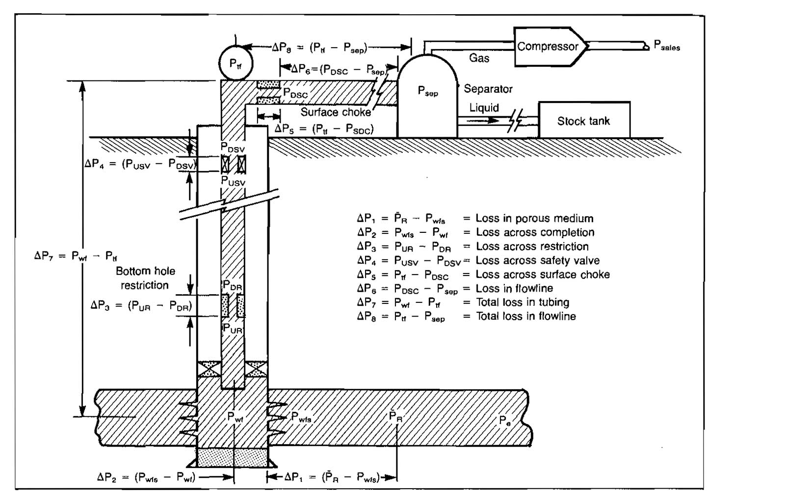
- Porous medium.
- Gravel pack or perforations.
- Bottom-hole choke.
- Well tubing.
- Subsurface safety valve (SSSV).
- Surface choke.
- Well flowline.
- Separator pressure.
- Flowline from compressor to sales line.
- Sales line pressure.
Procedures to calculate the pressure drop or resistance to flow in the porous medium and gravel pack are given in Manual for Engineers to Calculate Amount of Gas in Reservoirs“Essential Calculations of the Gas Reservoir Performance”. Pressure drops in all of the other restrictions may be calculated using the material in Performance of the Network of Pipes in Gas Industry“Performance of Piping System in the Modern Gas Industry”. The selection of a compressor to create the necessary pressure gain in the system can be made using information given in Usage of Natural Gas Compressors in the Gas Production Operations“Types and Design of the Natural Gas Compressors”.
Although all of these separate components of the production system can be analyzed independently, in order to determine the performance of the well they must be combined in a total system or nodal analysis. This is most easily accomplished by dividing the total system into two separate subsystems and determining the effects of changes made in one or both of the subsystems on the well performance. Selection of a location or node at which to divide the system depends on the purpose of the analysis. It is usually more convenient to select the division point at or as close as possible to the part of the system being analyzed.
For example, if the effect of subsurface safety valve size is being analyzed, the system is divided at the SSSV.
Picture 2 illustrates some of the most commonly used division points or nodes.

The analysis is accomplished by determining and plotting flow rate versus pressure existing at the division point or node for each of the subsystems. These are plotted as separate and independent curves on the same graph, and since there can be only one pressure existing at the division point, the intersection of the two subsystem curves gives the total system performance or flow rate, which will satisfy the requirement that the flow into the node must equal the flow out of the node. If the component being analyzed must be sized according to the flow rate and pressure change across the component, such as a SSSV or compressor, it is often convenient to plot pressure difference between the two subsystems versus flow rate. The system analysis procedures will be illustrated in this article in the form of example calculations.
Tubing and Flowline Size Effect
The size of piping installed in a well can have a large effect on the flow capacity or deliverability of the well. In some cases it can be the controlling factor and can cause the well to produce at a low rate even though the reservoir may be capable of producing much more gas.
Constant Wellhead Pressure
The simplest case will be considered first, that is, the case of a constant wellhead pressure. This case might occur if the well has a very short flowline between the wellhead and separator. In this case the well is divided at the bottom of the hole, node 6. The expressions for the inflow and outflow are.
Inflow:
Outflow:
The solution procedure is:
- Assume various values of pwf and determine qsc from inflow performance methods.
- Plot pwf versus qsc.
- Assume various flow rates, and starting at the fixed wellhead pressure, calculate pwf for each qsc using “Equation 27” or the Cullender and Smith method “Equation 29”.
- Plot pwf versus qsc on the same graph as in Step 2. The intersection of the curves gives the flow capacity and pwf for this particular tubing size.
To determine the effect of other tubing sizes, Steps 3 and 4 can be repeated for various tubing sizes. The effect of pwf can also be determined by repeating for various wellhead pressures. For this case, the two subsystems are:
- The reservoir and;
- The tubing plus the wellhead
pressure.
Example 1:
A stabilized deliverability test was conducted on a gas well to obtain reservoir inflow performance data. Determine the flow capacity of the well for both 1,995 in. and 2,441 ID tubing if pwf is constant at 1 000 psia. Other data are:
- n = 0,83;
- C = 0,0295 Mscfd/psia2;
- = 1 952 psia;
- H = 10 000 ft.
Solution:
The equation for generating the reservoir inflow performance curve is:
(This is the same well as was analyzed in “Manual for Engineers to Calculate Amount of Gas in Reservoirs – Example”).
- Assume various values of pwf and calculate qsc:
Inflow pwf, psia qsc, Mscfd 1 952 0 1 800 1 768 1 400 4 695 1 000 6 642 600 7 875 200 8 477 0 8 551 - Plot pwf versus qsc (Pic. 3).
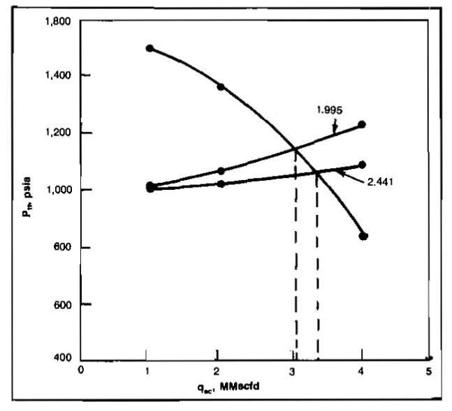
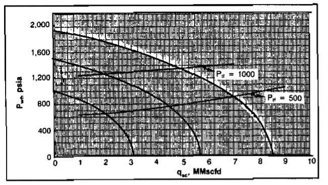
- Assume various flow rates and find the value of pwf required to overcome the pressure drop in the tubing and the wellhead pressure for each flow rate. This is required for each tubing size. For illustration purposes, the values of pwf are obtained from Performance of the Network of Pipes in Gas Industry“Picture – Vertical flowing gas gradients” and Performance of the Network of Pipes in Gas Industry“Picture – Vertical flowing gas gradients 2”. For more accuracy, that wall flow equations should be used.
Outflow pwf, psia qsc, Mscfd d = 1,995 d = 2,441 1 000 1 300 1 290 2 000 1 370 1 300 3 000 1 500 1 370 4 000 1 620 1 400 5 000 1 800 1 580 6 000 1 970 1 620 - Plot pwf versus qsc for both tubing strings on Picture 3. The only value of pwf that will satisfy both subsystems is the intersection of the inflow curve with the tubing performance curves. This occurs at the following values:
Tubing ID pwf, psia qsc, Mscfd 1,995 1 560 3 500 2,441 1 440 4 350 Thus, by installing the larger tubing, the well’s flow capacity can be increased by 850 Mscfd or about a 24 % increase.
Variable Wellhead Pressure
If a well is equipped with a flowline of considerable length, the size of the flowline can affect the flow capacity of the system. When flowline size effect is being considered, it is convenient to divide the system at the wellhead into two subsystems:
- The reservoir plus the tubing and;
- The flowline plus the separator pressure.
The inflow and outflow expressions are:
Inflow:
Outflow:
The solution procedure is:
- Assume various values of qsc and determine the corresponding pwf from inflow performance methods.
- Using the tubing pressure drop equations, determine the wellhead pressure, ptf corresponding to each qsc and pwf determined in Step 1.
- Plot ptf versus qsc.
- Using a fixed separator pressure and the pipeline flow equations, calculate ptf for several assumed flow rates.
- Plot ptf versus qsc on the same graph as used in Step 3. The intersection gives the only values of ptf and qsc that will satisfy both subsystems.
Example 2:
A 10 000 ft vertical well is equipped with 1,995 ID tubing and a 6 000 ft flowline. Separator pressure is fixed at 1 000 psia. Using the following data, determine the flow capacity for the system for both a 1,995 ID flowline and a 2,441 ID flowline.
- γg = 0,67;
- TR = 220 °F;
- Ttf = 100 °F;
- Tsep = 60 °F;
- μg = 0,012 cp;
- ∈ = 0,0018 in;
- n = 0,83;
- = 0,95;
- C = 0,0295 Mscfd/psia1,86;
- = 1 952 psia.
Solution:
- The reservoir inflow performance equation is:
or:
Assuming flow rates of 1, 2, 3, and 4 MMscfd, calculate the corresponding values of pwf. These values are given in the table at the end of the solution.
- The average pressure and temperature method was used to calculate ptf for each qsc and pwf. The equation is:
The values of ptf are given in the table.
- The values for each qsc and ptf for the reservoir-tubing subsystem are plotted on Picture 4.

Pic. 4 Example 2 Solution - The same flow rates as assumed in Step 1 are used to calculate ptf at a fixed psep of 1 000 psia for both the 1,995 and 2,441 in flowlines. The equation used is:
These values are also given in the table.
- The values for qsc and ptf for each line size for the flowline-separator subsystem are also plotted on Picture 4. The intersections with the reservoir-tubing line give flow capacities of 3 080 and 3 360 Mscfd for the 1,995 and 2,441 in. flowlines, respectively.
Inflow Outflow qsc, Mscfd pwf ptf (tubing) ptf (1,995) ptf (2,441) 1 000 1 877 1 500 1 016 1 006 2 000 1 774 1 362 1 062 1 022 3 000 1 653 1 158 1 134 1 049 4 000 1 512 840 1 227 1 085
Separator Pressure Effect
The effect of separator pressure on the system deliverability can best be determined by dividing the system at the separator. The subsystems then consist of:
- The separator and;
- The combination of the reservoir, the tubing, and the flowline.
The solution is obtained by plotting qsc versus psep, with psep calculated as:
The solution procedure is illustrated by reworking Example 2 using the 1,995 in. flowline.
- Calculate pwf for various qsc using the reservoir inflow equation.
- Calculate ptf for each pwf and qsc using Performance of the Network of Pipes in Gas Industry “Equation 27” Cullender and Smith.
- Calculate psep for each ptf and qsc “Equation 35” or “Equation 37”.
- Plot psep versus qsc and determine qsc for various values of psep.
Example 3:
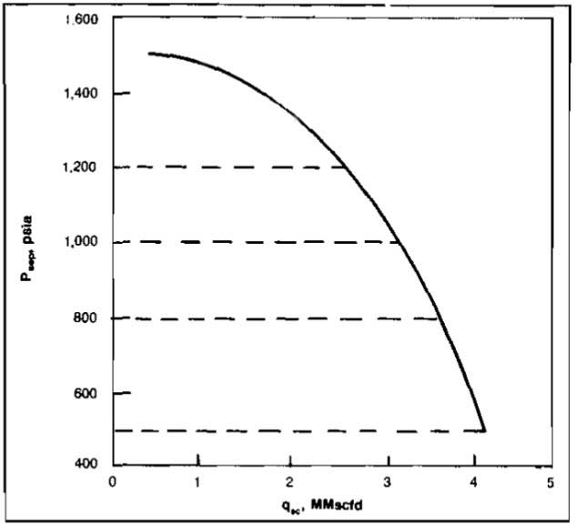
Determine the flow capacity for the well system of Example 2 for the 1,995 in flowline at separator pressures of 1 200, 1 000, 800, and 500 psia.
Solution:
The separator pressures are tabulated in the following table and plotted in Picture 5. The flow capacities for the various separator pressures are listed below.
| qsc, Mscfd | pwf | ptf | psep |
|---|---|---|---|
| 1 000 | 1 877 | 1 500 | 1 490 |
| 2 000 | 1 774 | 1 362 | 1 320 |
| 3 000 | 1 653 | 1 158 | 1 042 |
| 4 000 | 1 512 | 840 | 504 |
| psep | Flow capacity, Mscfd |
|---|---|
| 1 200 | 2 560 |
| 1 000 | 3 080 |
| 800 | 3 540 |
| 500 | 4 000 |
Compressor Selection
The selection or sizing of a compressor to increase the deliverability of a well system requires knowing the required suction and discharge pressures and the volume of gas to be pumped. The sales line pressure is usually fixed, but the gas may have to travel a considerable distance from the compressor to the sales line. The compressor discharge pressure would therefore be a function of gas flow rate. Compressor sizing is best accomplished by dividing the system at the compressor, or at the separator if the compressor is to be located near the separator.
The following procedure may be used to determine the necessary design parameters and power required to deliver a quantity of gas to a fixed sales line pressure.
Starting at
, determine
for various values of qsc using the procedure for determining separator pressure effect.
- Plot psep versus qsc.
- Starting at the sales line pressure, determine the discharge pressure required at the compressor, pdis. for various flow rates.
- Plot pdis. versus qsc on the same graph as used in Step 2. The intersection of these curves (if there is one) gives the flow capacity or deliverability for no compressor in the system.
- Select values of qsc and determine the values of p.dis, psep and Δp = pdis.-psep for each qsc.
- Calculate the required compression ratio, r = p.dis/psep and the power required using “Equation 9”.
Example 4:
The well system described in Examples 2 and 3 is to deliver gas to a sales line pressure of 1 000 psia through a 3,068 in. ID pipeline. The compressor is located at the separator, 10 000 ft from the sales line. Determine the compression ratio and horsepower required for delivery rates of 3,5 and 4,0 MMscfd.
Solution:
The separator or compressor suction pressures for various flow rates were calculated in Example 3 and plotted on Picture 5. These are replotted on Picture 6. Starting at the sales line pressure of 1 000 psia, the following required compressor discharge pressures were calculated using “Equation 35”.
| qsc, Mscfd | pdis, psia |
|---|---|
| 1 000 | 1 002 |
| 2 000 | 1 010 |
| 3 000 | 1 021 |
| 4 000 | 1 037 |
| 5 000 | 1 057 |
Plotting these points on Picture 6 gives an intersection at qsc = 3 040 for no compressor. The following values are read from Picture 6 at the flow rates of interest:
| qsc, Mscfd | psep | pdis | r = pdis/psep | Z1 |
|---|---|---|---|---|
| 3 500 | 810 | 1 030 | 1,27 | 0,86 |
| 4 000 | 500 | 1 040 | 2,08 | 0,92 |
To calculate the horsepower required, use “Equation 9” with:
- k = 1,3;
- psc = 14,7 psia;
- Tsc = 520 °R;
- T1 = 540 °R.
For qsc = 3 500 Mscfd:
For qsc = 4 000 Mscfd:
Subsurface Safety Valve Selection
Most offshore wells will require that some type of subsurface safety valve (SSSV) be installed in order to shut the well in if the wellhead pressure becomes too low. These may be velocity actuated or surface actuated type. In any event, unless the valve is tubing retrievable, it will not be full-opening and will therefore create a restriction to the well’s flow capacity. In order to select the appropriate SSSV, the well system is divided at the SSSV, Node 4 in Picture 2, The two subsystems are then:
- The reservoir plus the tubing below the SSSV and;
- The separator, flowline, surface choke, and the tubing above the SSSV.
The solution procedure is:
- Using the inflow performance and tubing equations, calculate the pressure upstream of the SSSV, pv1, for several flow rates.
- Plot pv1 versus qsc.
- Using the flowline equations, the surface choke equations if applicable, and the tubing equations, calculate the pressure downstream of the SSSV, pv2, for several flow rates.
- Plot pv2 versus qsc on the same graph. The intersection of the two curves gives the flow rate for no SSSV.
- Determine the Δp across the SSSV for several flow rates, Δp = pv1-pv2 and plot Δp versus qsc.
- Calculate the pressure drop across the SSSV for several qsc using “Equation 62”.
- Plot Δp versus qsc on the same graph as used in Step 5. The intersection of the two curves gives the flow capacity of the system for the particular size valve used in the calculations of Step 6. Repeat Steps 6 and 7 to determine the effect of SSSV size.
The solution could also be obtained by including the SSSV in the inflow expression. This would result in a different inflow curve for each SSSV size considered. The inflow and outflow expressions would be:
Inflow:
Outflow:
Example 5:
A 10 000 ft vertical well is to have a SSSV installed at a depth of 3 000 ft from the surface. The tubing size is 2,441 in. ID Other data are given in Example 2. Determine the flow capacity for SSSV’s having inside diameters of 0,4 in. and 0,5 in. The flowline diameter is also 2,441 in. ID.
Solution:
The well performance is tabulated below for the lower subsystem:
| qsc, Mscfd | pwf, psia | pv1, psia |
|---|---|---|
| 1 000 | 1 877 | 1 606 |
| 2 000 | 1 774 | 1 506 |
| 3 000 | 1 653 | 1 378 |
| 4 000 | 1 512 | 1 218 |
The performance for the upper subsystem is calculated by starting at a separator pressure of 1 000 psia:
| qsc, Mscfd | ptf, psia | pv2, psia |
|---|---|---|
| 1 000 | 1 006 | 1 088 |
| 2 000 | 1 022 | 1 113 |
| 3 000 | 1 049 | 1 154 |
| 4 000 | 1 085 | 1 209 |
The pressures above and below the SSSV are plotted versus qsc on Picture 7.
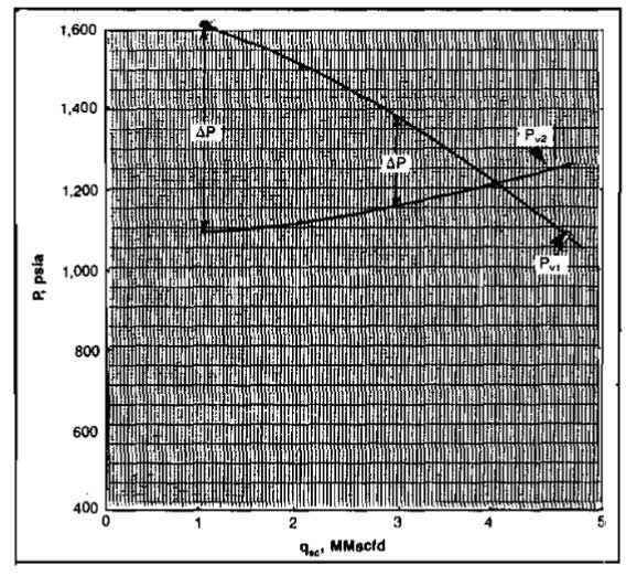
The intersection gives an unrestricted flow rate of 4 MMscfd. The pressure drop across the SSSV (pv1-pv2) is determined for several flow rates from Picture 7. The pressure drop for each flow rate and SSSV size is also calculated using “Equation 62” and plotted on Picture 8.
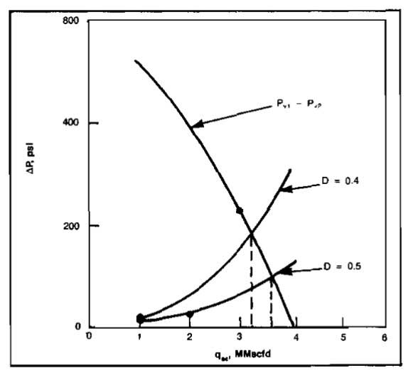
These are tabulated below. An example calculation of Δp using Equation below is presented for the 0,5 in. SSSV using:
- Cd = 0,9 and;
- Y = 0,85 for a flow rate of 2 MMscfd.
| Δp, psi | ||||
|---|---|---|---|---|
| qsc, Mscfd | pv1, psia | pv1-pv2 | D = 0,4 | D = 0,5 |
| 1 000 | 1 606 | 518 | 15 | 6 |
| 2 000 | 1 506 | 393 | 62 | 25 |
| 3 000 | 1 378 | 224 | 152 | 62 |
| 4 000 | 1 218 | 9 | 306 | 125 |
The results are obtained from Picture 8. The intersections of the Δp curves indicate flow capacities of 3 230 and 3 600 Mscfd for the 0,4 and 0,5 in. SSSV’s respectively.
Effect of Perforating Density
In many areas of the world, especially the Gulf Coast region of the United States, high capacity gas wells are completed in unconsolidated, high permeability formations. In order to control production of sand, the wells are completed by gravel packing. The flow capacity of the well may be controlled by the number of perforations, since the actual reservoir flow capacity is extremely high.
Another consideration in the well completion design is the pressure drop across the gravel pack. If it is too large, the gravel pack may be destroyed. The consensus is that this pressure drop should be less than about 300 psi, which means that the number of perforations required to meet this limit must be determined.
The method of analysis is the same as that used to analyze subsurface safety valve effect, except that the system is divided at the perforations. The equation for determining the Δp across the gravel pack was given in “Equation 94”.
The two subsystems are:
- The reservoir, including any actual skin damage and;
- The separator, flow line, surface choke, SSSV, and tubing.
The solution procedure is:
- Using the reservoir gas flow equation (Eq. 3-11), determine the pressure at the sandface, upstream of the gravel pack, pwfs for various flow rates, qsc.
- Plot pwfs versus qsc.
- Starting at the separator pressure, determine the bottom-hole flowing pressure required for the upper subsystem, pwf for various flow rates, qsc.
- Plot pwf versus qsc on the same graph as used in Step 2.
- Read values of pwfs and pwf at various qsc and plot Δp1 = pwfs-pwf versus qsc.
- Assume various qsc and calculate the pressure drop across the gravel pack, Δp2 using “Equation 94”. This should be done for various perforating densities.
- Plot Δp2 versus qsc on the same graph as used in Step 5. The intersection of the curves gives the flow capacity and the gravel pack pressure drop for various perforating densities.
Example 6:
The following data apply to the gas well shown in Picture 9 (see pics. 10 and 11 for solution).
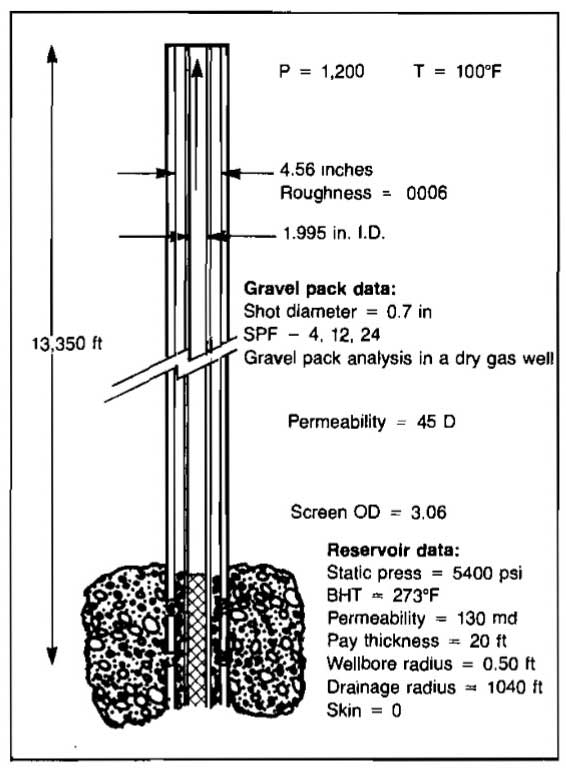
Determine the flow capacities and gravel pack pressure drops for 4, 12, and 24 perforations per foot for both 1,995 and 2,441 in. tubing.
- ptf = 1 200 psia;
- Ts = 100 °F;
- γg = 0,82;
- ∈ = 0,0006 in.;
- H = 13 350 ft;
- TR = 273 °F;
- μg = 0,012 cp;
- rθ = 1 040 ft;
- rw = 0,50 ft;
- S = 0;
- = 5 400 psia;
- h = 20 ft;
- Perforation diameter = 0,7 in.;
- = .97.
- Formation permeability = 130 md;
- Gravel permeability = 45 darcys;
- Screen outside diameter = 3,06 in;
- Hole diameter = 12,25 in.;
- N = (spf)h = (spf)(20).
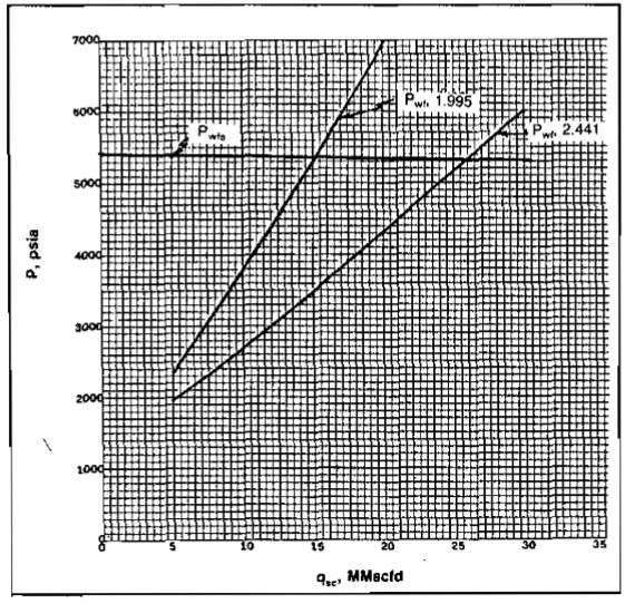
Solution:
1 Calculation of pwfs:
2
| qsc, Mscfd | pwfs, psia |
|---|---|
| 5 000 | 5 384 |
| 10 000 | 5 364 |
| 20 000 | 5 317 |
| 30 000 | 5 257 |
3 “Equation 27” is used to calculate pwf using a fixed ptf of 1 200 psia.
4
| pwf, psia | ||
|---|---|---|
| qsc, Mscfd | d = 1,995 | d = 2,441 |
| 5 000 | 2 385 | 1 974 |
| 10 000 | 3 786 | 2 606 |
| 15 000 | 5 358 | 3 405 |
| 20 000 | 6 987 | 4 168 |
| 30 000 | 10 080 | 5 998 |
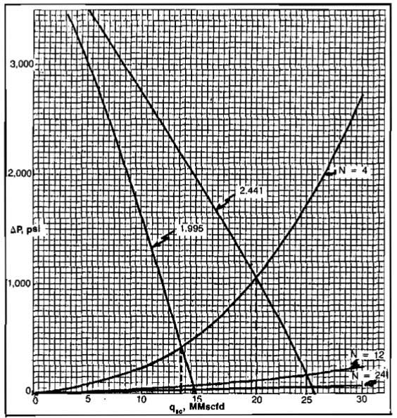
5
| Δp1, psi | ||
|---|---|---|
| qsc, Mscfd | d = 1,995 | d = 2,441 |
| 25 000 | – | 170 |
| 20 000 | – | 1 170 |
| 15 000 | 0 | 1 900 |
| 10 000 | 1 580 | 2 760 |
| 5 000 | 3 000 | 3 410 |
6 Calculation of pressure drop across the gravel pack for 4, 12, and 24 shots per foot:
7
| Δp2, psi | ||||
|---|---|---|---|---|
| qsc, Mscfd | pwfs, psia | N = 80 | N = 240 | N = 480 |
| 30 000 | 5 257 | 3 058 | 248 | 62 |
| 20 000 | 5 317 | 1 061 | 108 | 27 |
| 15 000 | 5 342 | 566 | 61 | 15 |
| 10 000 | 5 364 | 244 | 27 | 7 |
| 5 000 | 5 384 | 60 | 7 | 2 |
The results of the system analysis are tabulated below:
| Flow Capacity, Mscfd | |||
|---|---|---|---|
| Tubing ID | SPF = 4 | SPF = 12 | SPF = 24 |
| 1,995 | 13 700 | 14 500 | 14 600 |
| 2,441 | 21 000 | 25 000 | 26 000 |
The results show that the well is severely restricted by the smaller tubing size. The only reason for shooting more than 4 shots per foot if the small tubing is used is to reduce the pressure drop across the gravel pack to less than 300 psi. If the larger tubing is used, 12 shots per foot would be sufficient, giving a rate of 25 MMscfd at a pressure drop across the gravel pack of about 170 psi.
The inflow performance of this well would certainly justify tubing larger than the 2,441 size.
The analysis for determining the effect of perforating density on deliverability can also be performed by selecting other nodes. For example, if pwf were selected as the node pressure the inflow expression would include the pressure drop across the perforations. This would be calculated using “Equation 88” for gravel packed completions with AP and BP equal to zero.
When placing a newly gravel packed well on production it is advisable to be sure that the critical drop across the pack (approximately 300 psi) not be exceeded. This can be accomplished by calculating the expected wellhead pressure for various perforating densities and production rates and plotting ptf versus qsc. The wellhead pressure is obtained from:
A plot of ptf versus qsc for various perforating densities is illustrated in Picture 12. The values of flow rate at which the critical pressure drop is exceeded can be obtained from the plot of Δp versus qsc (Pic. 11). The actual wellhead pressure can be measured as the well’s rate is increased and plotted on Picture 12.
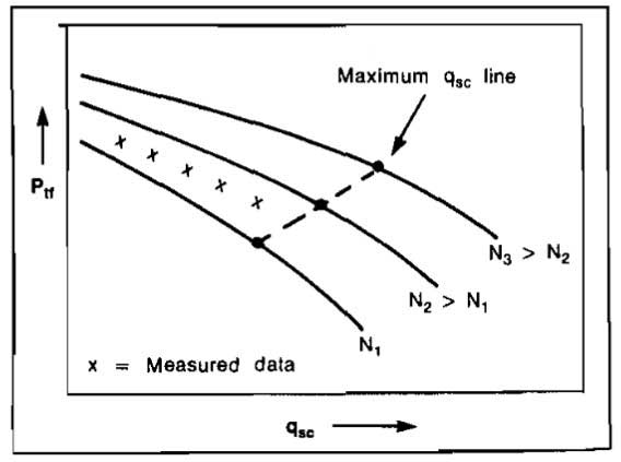
This will indicate the number of perforations that are effective and also allow the operator to determine the maximum rate at which he may produce the well without damaging the gravel pack.
Effect of Depletion
All of the previous analyses were performed at a constant reservoir pressure,
, that is at a particular time in the life of the reservoir. As gas is produced and
declines, the deliverability of the total system will decline. In order to maintain production at a constant rate, the flowing bottom-hole pressure pwf must be reduced as
declines. This can be accomplished by installing a compressor to lower separator pressure or by installing a larger flowline and ‘tubing to reduce the pressure drop in the piping system.
Inflow performance curves for declining
are illustrated in Manual for Engineers to Calculate Amount of Gas in Reservoirs“Inflow performance curve” for the reservoir described in “Manual for Engineers to Calculate Amount of Gas in Reservoirs – Example”. The decline in flow capacity for a given piping system can be determined by plotting the piping system performance on the same graph. The intersections give the flow capacity at various times as the reservoir pressure declines.
The following example illustrates how reducing the separator or wellhead pressure can help to maintain the deliverability as depletion occurs.
Example 7:
Determine the deliverability of the well described in Example 3-7 at values of
= 1 952, 1 500, and 1 000 psia at wellhead pressures of 1 000 and 500 psia if the well is equipped with 3,5 in. (2,992 ID) tubing. Other data are:
- H = 10 000 ft;
- γg = 0,67;
- = 160 °F;
- μg = 0,012 cp;
- ∈ = 0,0018 in.
Solution:
The system is divided at the sandface. The inflow performance was calculated in “Manual for Engineers to Calculate Amount of Gas in Reservoirs – Example” and is replotted in Picture 13. The values of pwf for the upper subsystem are tabulated below and plotted on Pic. 13. The flow capacities are also tabulated.
| pwf, psia | ||
|---|---|---|
| qsc, Mscfd | ptf = 1 000 | ptf = 500 |
| 1 000 | 1 256 | 635 |
| 3 000 | 1 283 | 685 |
| 5 000 | 1 337 | 780 |
| 7 000 | 1 415 | 905 |
| 9 000 | 1 510 | 1 045 |
| Flow Capacity, Mscfd | ||
|---|---|---|
| ptf = 1 000 | ptf = 500 | |
| 1 952 | 4 950 | 7 000 |
| 1 500 | 1 950 | 4 500 |
| 1 000 | – | 1 975 |
Relating Performance to Time
The deliverability or producing capacity of a well or field with respect to time must be known for economic evaluations and for planning equipment purchases. The producing capacity depends on the average reservoir pressure
, which is a function of the cumulative gas produced, Gp. Also, the time required to produce a quantity of gas, ΔGp , depends on the flow capacity, qsc, during the time period. At in which the gas was produced. If the production rate is restricted by allowable, the rate of increase in Gp will be constant until the producing capacity drops below the allowable rate.
Prediction of the rate versus time and cumulative production versus time requires plots of
or
/Z versus Gp and
versus qsc. A plot of
/Z or
versus Gp is obtained from a material balance calculation, as described in Manual for Engineers to Calculate Amount of Gas in Reservoirs“Essential Calculations of the Gas Reservoir Performance”.
The procedure involves selecting time periods small enough such that
can be considered constant during the period. The smaller the time period, or the smaller the value of ΔGp selected, the more accurate the prediction will be. The procedure is:
Construct graphs of
versus
Gp and
versus qsc (Pic. 14).
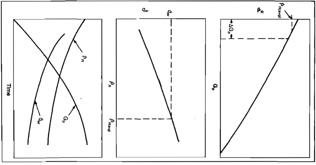

Pic. 14 Relating performance to time Select a small quantity of gas produced, ΔGp and determine the average value of
applicable during this interval from the
versus Gp plot.
From the plot of
versus qsc, find the average production rate,
, corresponding to the average
found in Step 2.
- Calculate the time interval required to produce ΔGp from:
Calculate t = ΣΔt and Gp = ΣΔGp. Plot Gp,
and qsc versus t. Repeat until the economic limit is reached.
Nodal Analysis of Injection Wells
All of the previous examples in this chapter have dealt with flowing production wells. The production engineer must sometimes design completion configurations for or analyze performance of various types of injection wells. These wells may be used for injecting gas in gas storage reservoirs. Nodal analysis may be performed on injection wells by selecting the node at bottomhole such that the inflow to the node will include the compressor and the piping system, while the outflow will consist of the perforations and reservoir. For example, if gas from a compressor is being injected into a well, the inflow and outflow expressions would be:
Inflow:
Outflow:
This type of analysis could be used to determine the effects on injection rate of various compressor pressures, flowline sizes or tubing sizes. The effect of tubing size on injection rate will be illustrated by an example. For this example it is assumed that wellhead pressure is Constant so that the inflow will include only the pressure drop in the tubing. That is:
Inflow:
“Equation 27” may be used to calculate pwf for various rates. The outflow performance may be calculated using the back-pressure equation for gas wells. That is:
Outflow:
where:
or:
Example 8:
Using the following data determine the rate at which gas can be injected into this well for 2-3/8 in., 2-7/8 in., and 3-1/2 in. tubing.
- = 2 000 psia;
- Injection pwh = 4 000 psia;
- γg = 0,7;
- Twh = 150 °F;
- Tres = 150 °F;
- well depth = 10 000 ft;
- ∈ = 0,0018 in.
From a previous injection test:
Solution:
The inflow performance can be calculated from:
where:
The solution for pwf for any injection rate will be iterative since
depends on the average of pwf and pwh. The iterative procedure will be illustrated for one tubing size and one rate. If a computer is available the tubing can be divided into short increments of length and the solution will be more accurate. The procedure for hand calculations is:
- Assume a value for pwf.
Calculate
Calculate
and
at
- Calculate pwf and compare with the assumed value. If not close, use the calculated pwf as next estimate and go to step 2.
The procedure will be illustrated by calculating the bottomhole pressure for the 2-3/8 (1,995) tubing for an injection rate of 4 MMscfd. For this rate:
| Assumed | Calculated | ||||||
|---|---|---|---|---|---|---|---|
| pwf | Z | μ | NRθ | f | S | pwf | |
| 4 000 | 4 000 | .879 | .025 | 1,12·106 | .019 | .489 | 4 991 |
| 4 991 | 4 496 | .921 | .027 | 1,04·106 | .019 | .467 | 4 930 |
| 4 930 | 4 465 | .918 | .027 | 1,04·106 | .019 | .469 | 4 934 |
| 4 934 | 4 467 | .918 | .027 | 1,04·106 | .019 | .469 | 4 934 |
This procedure was followed for the various injection rates and tubing sizes in order to produce the following table of inflow pressures and rates:
| Inflow | |||
|---|---|---|---|
| Injection Rate MMscfd | pwf, psia | ||
| 2-3/8 tubing | 2-7/8 tubing | 3-1/2 tubing | |
| 0 | 5 050 | 5 050 | 5 050 |
| 4 | 4 934 | 5 010 | 5 035 |
| 8 | 4 580 | 4 890 | 4 995 |
| 12 | 3 945 | 4 685 | 4 925 |
| 16 | 2 910 | 4 390 | 4 830 |
| 20 | 1 200 | 3 985 | 4 700 |
| 24 | 0 | 3 455 | 4 540 |
| 28 | 0 | 2 735 | 4 350 |
| 32 | 0 | 1 900 | 4 120 |
The reservoir or outflow performance is calculated from:
| Outflow | |
|---|---|
| Injection Rate MMscfd | pwf, psia |
| 0 | 2 000 |
| 4 | 2 336 |
| 8 | 2 695 |
| 12 | 3 039 |
| 16 | 3 363 |
| 20 | 3 671 |
| 24 | 3 964 |
| 28 | 4 245 |
| 32 | 4 514 |
The intersections of the various inflow curves with the outflow curve in Picture 15 represent the injection rates possible for the 3 tubing sizes. The results are tabulated below:
| Tubing Size, inches | Injection Rate, MMscfd |
|---|---|
| 2-3/8 | 14,6 |
| 2-7/8 | 21,5 |
| 3-1/2 | 29 |
This well could also be analyzed for other wellhead pressures. In gas storage operations the static reservoir pressure will increase as gas is injected and this would cause an upward shift in the outflow curve in Picture 15.
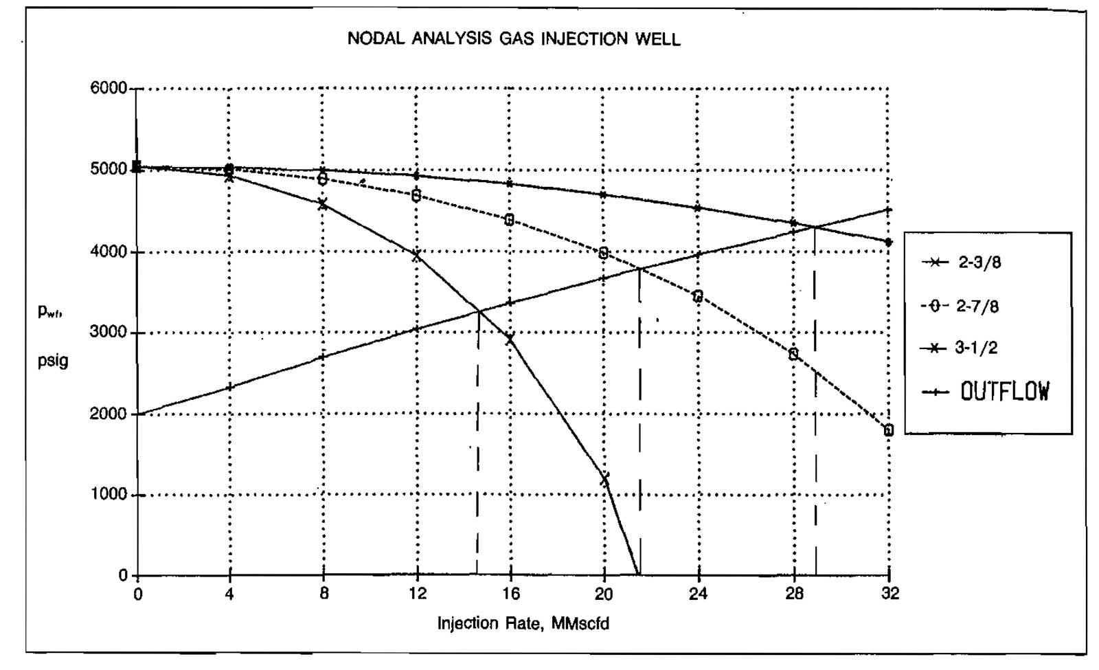
This would result in a decreasing injection rate with time, as the intersection of the inflow and outflow curves would shift to the left. The change in injection rate with time could be determined by using a procedure similar to that discussed in the previous section.
Analyzing Multiwell Systems
The concepts discussed for applying total system or nodal analysis to single wells can also be applied to the analysis of multiwell systems, including entire fields. The procedure will be illustrated qualitatively by referring to the simple system shown in Picture 16. In this case a change made in any component in the system would affect the producing capacity of the total system. Some of the changes which could be considered are:
- Working over individual wells.
- Adding new wells to the system.
- Shutting in some of the existing wells.
- Changes in producing characteristics with time.
- Effect of surface line sizes.
- Installation of compressors.
- Effect of the final outlet pressure, pD.
The location of the node for the final analysis must be selected at a point such that there is no further commingling of flow streams downstream of the node. For the system shown in Picture 16 this would be at either point C or point D.
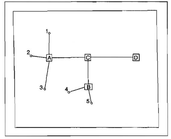
Intermediate nodes must be selected at any point where flow streams commingle upstream of the final node, points A and B in the system shown. The analysis must begin at the reservoir pressure which is independent of rate and end at some final outlet pressure which is also independent of rate.
To illustrate the procedure consideration will be given to either changing the pressure at point D or looping the surface line between points C and D. The node will be selected at point C. Intermediate nodes must be considered at points A and B.
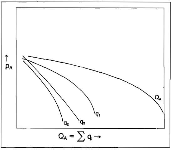
The inflow to point A will be calculated from:
This expression would be evaluated for each well feeding into point A for a range of producing rates. This would result in a plot such as illustrated in Picture 17.
A similar plot for the pressure behavior at point B can be constructed by considering wells 4 and 5. This is illustrated in Picture 18.

The gas-liquid ratios and water fractions used in calculating the pressure drops in the piping system to this point would be those corresponding to the individual wells, since no commingling of well streams has occurred.
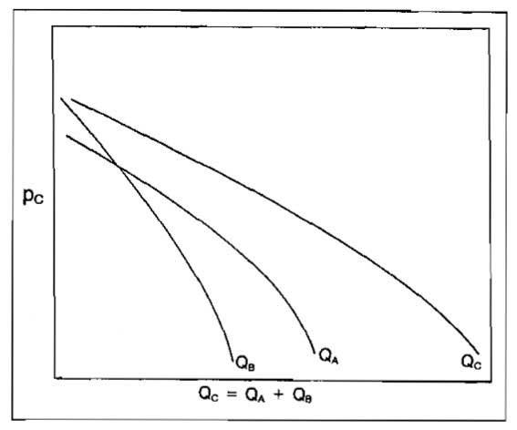
Moving downstream to the next point at which commingling occurs, point C, the inflow expressions for the flows coming from points A and B are:
and:
This will result in a relationship between pressure at point C and the inflow rate into point C as illustrated in Picture 19.
The calculation of the pressure drops between points A and C, ΔpAC and between points B and C, ΔpBC is complicated by the fact that the GLR and water fractions are functions of rate if the individual wells have different values of these parameters. In this case the correct GLR and fw for each commingled rate are calculated using:
and:
Similar expressions are used to determine these values for calculating ΔpBC.
The expression for the outflow from point C is:
Calculation of ΔpCD for various rates would again require determining the correct GLR and fw corresponding to each Qc = QA+QB. A change in either PD or the line size between points C and D would result in different outflow curves and thus different system capacities, as shown in Picture 20.
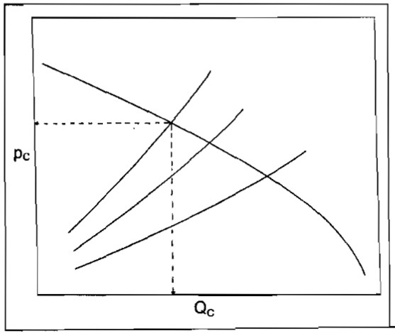
To determine the effect of these changes on individual well performance, the pressure at point C corresponding to an intersection on Picture 20 can be used to move upstream to points A and Band thus determine the individual well rates.
The procedure outlined above will also apply if some of the wells are under choke control. If a well is flowing through a choke in critical flow, the well’s rate will be constant unless the pressure downstream of the choke is increased to the point at which critical flow no longer occurs.
Summary
The procedures and examples presented in this article demonstrate how the effect of any variable in the total well system may be isolated and analyzed. This was accomplished by dividing the total system into two subsystems, the division being made at various points or nodes, usually as close as possible to the component being considered.
Even though each subsystem is analyzed separately, any change in a component of the subsystem affects the total system performance, therefore, to obtain any meaningful design parameters, this method should be used.