Essential Calculations of the Gas Reservoir Performance

In traveling from its original location in the reservoir to the final point of consumption, the gas must first travel through the reservoir rock or porous medium. A certain amount of energy is required to overcome the resistance to flow through the rock, which is manifested in a pressure decrease in the direction of flow, toward the well. This pressure drop or decrease depends on the gas flow rate, properties of the reservoir fluids, and properties of the rock. The fluid properties were discussed in Best and Most Widely Methods to Perform Necessary Calculations with a Gas“Methods to Made Calculation of a Gas Producing System”, and a brief discussion of the rock properties is given in this article.

СодержаниеСвернуть

Reservoir Gas Flow
Flow Regime Characteristics
Flow Equations
Well Deliverability or Capacity
Transient Testing
Real Gas Pseudo-Pressure Analysis
Gas Reserves
Reserve Estimates – Volumetric Method
Reserve Estimates – Material Balance Method
Energy Plots
Abnormally Pressured Reservoirs
Well Completion Effects
Open-Hole Completions
Perforated Completions
Perforated, Gravel-Packed Completions
Tight Gas Well Analysis
Guidelines for Gas Well Testing
Sweet Dry Gas
Sweet Wet Gas
Sour Gas
Flow Measuring
Pressure Measuring
Test Design
Problems in Gas-Well Testing
Reporting Data

The engineer involved in gas production operations must be able to predict not only the rate at which a well or field will produce, but also how much gas is originally in the reservoir and how much of it can be recovered economically. This requires the ability to relate volumes of gas existing in the reservoir to reservoir pressure. Because the flow capacity of a well depends on the reservoir pressure, both reservoir gas flow and reserve estimates are discussed in this article.

Reservoir Gas Flow

Determination of the inflow performance or reservoir flow capacity for a gas well requires a relationship between flow rate coming into a well and the sand-face pressure or flowing bottom-hole pressure. This relationship may be established by the proper solution of Darcy’s Law, which is the accepted expression relating pressure drop and fluid velocity in a porous medium, provided that the flow is laminar. Solution of Darcy’s Law depends on the conditions of flow existing in the reservoir or the flow regime. The flow type or regime may be independent of time or steady-state, or if conditions at a particular location change with time, the flow regime is transient or unsteady-state. Under certain conditions of transient flow, conditions change at a constant rate at all locations in the reservoir. This condition is called pseudo-steady-state and may be analyzed more simply than the transient condition.

The flow regimes will be discussed qualitatively first, the equations for each regime will be presented, and then the application of the equations for determining inflow performance or well flow capacity will be presented.

Flow Regime Characteristics

When a well is opened to production from a shut-in condition, the pressure disturbance created at the well travels outward through the rock at a velocity governed by the rock and fluid properties. The various flow regimes are discussed with respect to the behavior of this pressure disturbance.

Steady-State Flow. Picture 1 illustrates the pressure and flow rate distribution occurring during radial, steady-state flow into a well. This pressure distribution will remain constant as long as the radius being drained by the well remains constant.

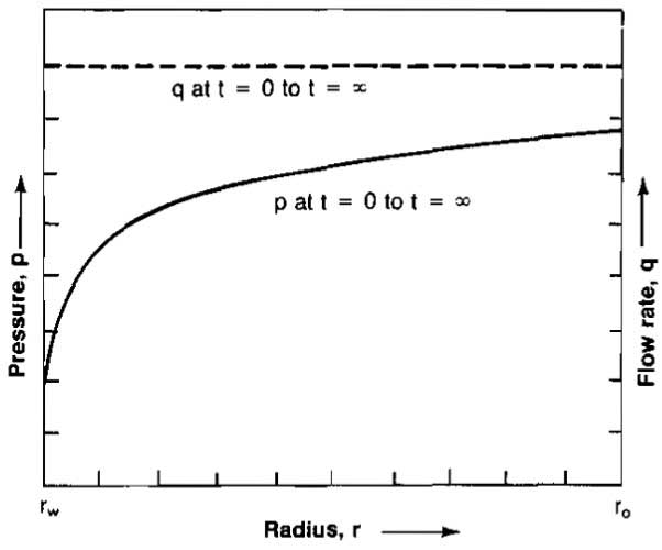
For such a situation to be strictly true it is necessary that the flow across the external drainage radius r_e be equal to the flow across the well radius at r_w. This is never sttictly met in a reservoir other than a strong water drive, whereby the water influx rate equals the producing rate. Pressure maintainance by water injection down-dip or by gas injection updip would also approximate steady-state conditions as would most pattern waterfloods after the initial stages of injection have passed.

Steady-state equations are also useful in analyzing the conditions near the wellbore because even in an unsteady-state system the flow rate near the wellbore is almost constant so that the conditions around the wellbore are almost constant. Thus, steady-state flow equations can be applied to this portion of the reservoir without any significant error.

Unsteady-State Flow. Picture 2 shows the pressure and rate distributions for a radial system at various times for a closed reservoir (no flow across r_e).

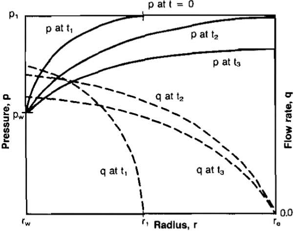
In this case all of the production is due to the expansion of the fluid in the reservoir. This causes the rate at r_e to be zero and the rate increases to a maximum at the well radius, r_w. In the steady-state case the flow across r_w, the well radius. With flow across r_e zero, the only energy causing the flow of fluid is the expansion of the fluids themselves. Initially the pressure is uniform throughout the reservoir at p_i. This represents the zero producing time.

The production rate is a controlled so that the pressure at the well is constant. A pressure distribution shown as p at t₁ is obtained after a short period of time of producing the well at such a rate that the well pressure remains constant. At this time only a small portion of the reservoir has been affected or has had a significant pressure drop.

For a closed reservoir, flow occurs due to expansion of the fluid. Consequently, if no pressure drop exists in the reservoir at a particular point, or outside of that point, no flow could be taking place at that particular radius. The fluid could not expand without a drop in pressure.

Thus, as shown in the plot of q at t₁ the rate at r_e is zero and increases with a reduction in radius until the maximum rate in the reservoir is obtained at r_w. The pressure and rate distribution at time t₁ represent an instant in time, and the pressure and rate distributions move on through these positions immediately as the production continues to affect more and more of the reservoir. That is, more and more of the reservoir continues to experience a significant pressure drop and is subjected to flow until the entire reservoir is affected as shown by the pressure at t₂. The rate, q, at t₂ indicates that the flow rate at this time extends throughout the reservoir since all of the reservoir has been affected and has had a significant pressure drop.

Notice that the rate at the well has declined somewhat from time t₁ to t₂ since the same pressure drop (p_i-p_w), is effective over a much larger volume of the reservoir. Once the pressure in the entire reservoir has been affected the pressure will drop throughout the reservoir as production continues so that the pressure distribution might be as shown for p at t₃. The rate will have declined somewhat during time t₁ to t₂ due to the increase in the radius over which flow is taking place, and it will continue to decline from t₂ to t₃ due to the decline of thc total pressure drop from r_e to r_w, (p_e-p_w).

Note that from time t = 0 to time t₂, when a pressure drop is finally affected throughout the entire reservoir, the pressure and rate distributions would not be affected by the size of the reservoir or the position of the external drainage radius r_e. During this time the reservoir is said to be infinite-acting because during this period the outer drainage radius r_e, could mathematically be infinite. Even in reservoir systems that are dominated by steady-state flow, the effect of changes in well rates or well pressures at the well will be governed by unsteady-state flow equations until the changes have been in effect for a sufficient length of time to affect the entire reservoir and have the reservoir again reach a steady-state condition.

Pseudo-Steady-State Flow. Picture 3 illustrates the pressure and rate distribution for the same unsteady-state system except that in this case the rate at the well, q_w, is held constant. This might be comparable to a prorated well or one that is pumping at a constant rate.

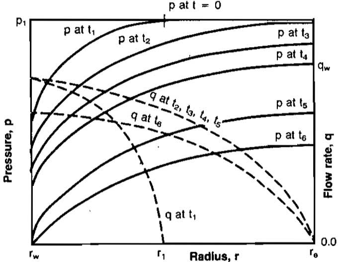
Again at time t = 0 the pressure throughout the reservoir is uniform at p_i. The after some short producing time t₁ at a constant rate, only a small portion of the reservoir will have experienced a significant pressure drop, and consequently the reservoir will be flowing only out to a radius r₁. As production continues at the constant rate, the
entire reservoir will eventually experience a significant pressure drop as shown at t₂. Shortly after the entire reservoir pressure has been affected, the change in the pressure with time at all radii in the reservoir becomes uniform so that the pressure distributions at subsequent times are parallel as illustrated by the pressure distributions at times t₃, t₄ and t₅. This situation will continue with con stant changes in pressure with time at all radii and with subsequent parallel pressure distributions until the reservoir is no longer able to sustain a constant flow rate at the wellbore. This will occur when the pressure at the well, p_w, has reached its physical lower limit.

Pseudo-steady-state flow occurs in the reservoir after it has been produced at a constant rate for a long enough period of time to cause a constant change in pressure at all radii, resulting in parallel pressure distributions and corresponding constant rate distributions. Pseudo-steady-state flow is a specialized case of unsteady-state flow and is sometimes referred to as stabilized flow. Most of the life of a reservoir will exist in pseudo-steady-state flow.

Flow Equations

From the previous description of the various flow regimes it is obvious that a particular well will be operating in each of these regimes at some time in the life of the well. The applicable equations for each flow regime will be derived or presented in this section.

Steady-State Flow

Darcy’s Law for flow in a porous medium is:

v = - \frac{k}{μ} \frac{d p}{d x} or q = v A = - \frac{k A}{μ} \frac{d p}{d x} E q . 1

where:

v = fluid velocity;
q = volumetric flow rate;
k = effective permeability;
μ = fluid viscosity, and;
$\frac{d p}{d x}$
= pressure gradient in the direction of flow.

For radial flow in which the distance is defined as positive moving away from the well, the equation becomes:

q = \frac{k (2 πrh)}{μ} \frac{d p}{d r} E q . 2

where:

r = radial distance, and;
h = reservoir thickness.

Darcy’s Law describes the pressure loss due to viscous shear occurring in the flowing fluid. If the formation is not horizontal, the hydrostatic or potential energy term must be included. This is usually negligible for gas flow in reservoirs. Equation 2 is a differential equation and must be integrated for application. Before integration the flow equation must be combined with an equation of state and the continuity equation. The continuity equation is:

ρ_{1} q_{1} = ρ_{2} q_{2} = c o n s t a n t E q . 3

From Best and Most Widely Methods to Perform Necessary Calculations with a Gas“Methods to Made Calculation of a Gas Producing System”, the equation of state for a real gas is:

ρ = \frac{p M}{Z R T} . E q . 4

The flow rate for a gas is usually desired at some standard conditions of pressure and temperature, p_sc and T_sc. Using these conditions in Equation 3 and combining Equations 3 and 4:

ρ q = ρ_{s c} q_{s c},

or:

q \frac{p M}{Z R T} = q_{s c} \frac{p_{s c} M}{Z_{s c} R T_{s c}} .

Solving for q_sc and expressing q with Equation 2 gives:

q_{s c} = \frac{p T_{s c}}{p_{s c} Z T} \frac{2 π r h k}{μ} \frac{d p}{d r}

The variables in this equation are p and r. Separating the variables and integrating:

\int_{p_{w}}^{p_{e}} p d p = \frac{q_{s c} p_{s c} T \bar{μ} \bar{Z}}{T_{s c} 2 π k h} \int_{r_{w}}^{r_{e}} \frac{d r}{r}

\frac{{p_{e}}^{2} - {p_{w}}^{2}}{2} = \frac{q_{s c} p_{s c} T \bar{μ} \bar{Z}}{T_{s c} 2 π k h} \ln (r_{e} / r_{w})

or:

q_{s c} = \frac{π k h T_{s c} ({p_{e}}^{2} - {p_{w}}^{2})}{p_{s c} T \bar{μ} \bar{Z} \ln (r_{e} / r_{w})} . E q . 5

In this derivation it was assumed that μ and Z were independent of pressure. They may be evaluated at reservoir temperature and average pressure in the drainage area:

\bar{p} = \frac{p_{e} + p_{w}}{2} .

Equation 5 is applicable for any consistent set of units. In so-called conventional oil field units the equation becomes:

q_{s c} = \frac{703 \cdot 10^{- 6} k h ({p_{e}}^{2} - {p_{w}}^{2})}{T \bar{μ} \bar{Z} \ln (r_{e} / r_{w})} E q . 6

where:

q_sc = Mscf/day;
k = permeability in millidarcies;
h = formation thickness in feet;
p_e = pressure at r_e, psia;
p_w = wellbore pressure at r_w, psia, and;
$\bar{μ}$
= gas viscosity, cp.

This equation incorporates the following values for standard pressure and temperature:

p_sc = 14,7 psia,

T_sc = 60 °F = 520 °R.

These units will be used in all equations in the text unless otherwise stated.

Example 1

Given the following data, determine the well bore pressure required for an inflow rate of 3 900 Mscfd assuming steady-state flow.

k = 1,5 md;
p_e = 4 625 psia;
T = 712 °R = 252 °F;
r_e = 550 ft;
h = 30 ft;
$\bar{μ}$
= 0,027 cp;
γ_g = 0,76;
r_w = 0,333 ft.

Solution:

The solution is iterative since:

\bar{Z} = f (\bar{p}),

where:

$\bar{p} = \frac{p_{e} + p_{w}}{2},$
and;
r_w is the unknown.

As a first estimate, assume

$\bar{Z}$

= 1,0.

First Trial

{p_{w}}^{2} = {p_{e}}^{2} - \frac{\bar{μ} T \ln (r_{e} / r_{w}) q_{s c} \bar{Z}}{703 \cdot 10^{- 6} k n}

{p_{w}}^{2} = 2, 139 \cdot 10^{7} - \frac{(0, 027) (712) (7, 41) (3 900) \bar{Z}}{703 \cdot 10^{- 6} (1, 5) (30)}

{p_{w}}^{2} = 2, 139 \cdot 10^{7} - 1, 756 \cdot 10^{7} \bar{Z} = 2, 139 \cdot 10^{7} - 1, 756 \cdot 10^{7} (1)

{p_{w}}^{2} = 3, 83 \cdot 10^{6} p_{w} = 1 957 p s i a

\bar{p} = \frac{4 625 + 1 957}{2} = 3 291 p s i a

Evaluation of

$\bar{Z}$

at 3 291 psia and 712 °R gives

$\bar{Z}$

= 0,88.

Second Trial

{p_{w}}^{2} = 2, 139 \cdot 10^{7} - 1, 756 \cdot 10^{7} (0, 88) = 5, 937 \cdot 10^{6}

p_{w} = 2 436 p s i a \bar{p} = 3 530 p s i a

At 3 530 psia and 712°R,

$\bar{Z}$

= 0,89.

Third Trial

{p_{w}}^{2} = 2, 139 \cdot 10^{7} - 1, 756 \cdot 10^{7} (0, 89) = 5, 762 \cdot 10^{6}

p_{w} = 2 400 p s i a \bar{p} = 3 512 p s i a \bar{Z} = 0, 89

Since the value for

$\bar{Z}$

is the same as for Trial 2, the solution has converged and the required well pressure is 2 400 psia. The solution would have been more complicated if a constant for μ had not been assumed.

The above treatment of steady-state flow assumes no turbulent flow in the formation and no formation or skin damage around the wellbore. The effects of turbulence and skin will be examined in a following section.

Although steady-state flow in a gas reservoir is seldom reached, the conditions around the wellbore can approach steady-state. The steady-state equation including turbulence is:

{p_{e}}^{2} - {p_{w}}^{2} = \frac{1 422 T \bar{μ} \bar{Z} q_{s c} \ln (r_{e} / r_{w})}{k h} . . . + \frac{3, 161 \cdot 10^{- 12} β γ_{g} \bar{Z} {q_{s c}}^{2} T}{h^{2}} (\frac{1}{r_{w}} - \frac{1}{r_{e}}) . E q . 7

or:

p_{e}^{2} - p_{w}^{2} = A q_{s c} + B q_{s c}^{2} E q . 7 (a)

where:

A = 1 422 T \bar{μ} \bar{Z} \ln (r_{e} / r_{w}) / k h

B = \frac{3, 161 \cdot 10^{- 12} β γ_{g} \bar{Z} T}{r_{w} h^{2}}

In the definition of the B term it was assumed that (1/r_e) is negligible compared to (1/r_w).

The first term on the right hand side is the pressure drop from laminar or Darcy flow, while the second term gives the additional pressure drop due to turbulence. If the fluid properties are known and the permeability is known from some source such as a drawdown test, the turbulent effects can be calculated using the results of a test. This will be used later to distinguish between actual formation damage and turbulence. Values of the velocity coefficient β for various permeabilities and porosities can be obtained from Picture 4 or calculated from Equation 8.

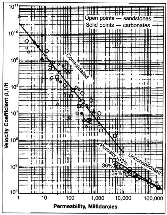
Values of velocity coefficient — Pic. 4 Gas velocity coefficient

β = \frac{2, 33 \cdot 10^{10}}{k^{1, 2}} E q . 8

where:

k – is millidarcies.

Pseudo-Steady-State Flow

An equation for pseudo-steady-state flow can be derived that will show that:

q_{s c} = \frac{703 \cdot 10^{- 6} k h ({\bar{p}}_{r}^{2} - {p_{w}}^{2})}{T \bar{μ} \bar{Z} \ln (0, 472 r_{e} / r_{w})} . E q . 9

Although time does not appear explicitly in Equation 9, it should be remembered that both

${\bar{p}}_{R}$

and p_w will be declining at the same rate for a constant q once the pressure disturbance has reached the reservoir boundary.

The effects of skin damage and turbulence are sometimes included in Equation 9 as follows:

q_{s c} = \frac{703 \cdot 10^{- 6} k h ({\bar{p}}_{r}^{2} - {p_{w}}^{2})}{T \bar{μ} \bar{Z} [\ln (. 472 r_{e} / r_{w}) + S + D q_{s c}]} E q . 10

where:

S = dimensionless skin factor, and;
D = turbulence coefficient.

It is frequently necessary to solve Equation 10 for pressure or pressure drop for a known q_sc.

{\bar{p}}_{R}^{2} - {p_{w}}^{2} = \frac{1 422 T \bar{μ} \bar{Z} [\ln (. 472 r_{e} / r_{w}) + S] q_{s c}}{k h} + \frac{1 422 T \bar{μ} \bar{Z} D q_{s c}^{2}}{k h}

or:

{\bar{p}}_{R}^{2} - p_{w}^{2} = A q_{s c} + B q_{s c}^{2}

A = \frac{1 422 T \bar{μ} \bar{Z} [\ln (. 472 r_{e} / r_{w}) + S]}{k h}

B = \frac{1 422 T \bar{μ} \bar{Z} D}{k h}

Unsteady-State Flow

It was stated earlier that any well flows in the unsteady-state or transient regime until the pressure disturbance reaches a reservoir boundary or until interference from other wells takes effect. Although the flow capacity of a well is desired for pseudo-steady-state or stabilized conditions, much useful information can be obtained from transient tests. This information includes permeability, skin factor, turbulence coefficient, and average reservoir pressure. The procedures are developed in the section on transient testing. The relationships among flow rate, pressure, and time will be presented in this section for various conditions of well performance and reservoir types. It will be seen that the steady-state and pseudo-steady-state equations can be obtained from solution of the diffusivity equation as special cases.

The diffusivity equation can be derived by combining an unsteady-state continuity equation with Darcy’s Law and the gas equation of state. The equation is:

\frac{\partial^{2} p^{2}}{\partial r^{2}} + \frac{1}{r} \frac{\partial p^{2}}{\partial r} = \frac{ϕ μ C}{k} \frac{\partial p^{2}}{\partial t} E q . 12

This equation can be solved for pressure as a function of flow rate and time, but the solutions and application of the solutions are simplified if the diffusivity equation is written in dimensionless form. This is accomplished by defining the following dimensionless variables:

The following units are to be used in calculating values for the dimensionless numbers in Table 1:

k = millidarcies;
t = hours;
μ = cp;
q_sc = Mscfd;
p = psia;
C = psi^-1;
r = ft;
T = °R;
h = ft.

Table 1. Dimensionless Variables
Dimensionless Variable	Symbol	Definition
Time	t_D	$\frac{2, 64 \cdot 10^{- 4} k t}{ϕ \bar{μ} \bar{C} r^{2}} E q . 13$
Radius	r_D	$\frac{r}{r_{w}} E q . 14$
Flow rate	q_D	$\frac{1 422 T q_{s c} \bar{Z} \bar{μ}}{k h p_{l}^{2}} E q . 15$
Pressure	p_D	$\frac{p^{2}}{p_{l}^{2} q_{D}} E q . 16$
Pressure drop	Δp_D	$\frac{p_{l}^{2} - p^{2}}{p_{l}^{2} q_{D}} E q . 17$

The diffusivity equation in dimensionless variables becomes:

\frac{\partial^{2} ∆ p_{D}}{\partial {r_{D}}^{2}} + \frac{1}{r_{D}} \frac{\partial ∆ p_{D}}{\partial r_{D}} = \frac{\partial ∆ p_{D}}{\partial t_{D}} . E q . 18

Solutions to Equation 18 depend on the reservoir type and boundary conditions. The following solutions will be presented:

Constant rate at well, infinite-acting reservoir (transient);
Constant rate at well, finite-acting (closed) reservoir (pseudo-steady-state);
Constant rate at well, constant pressure at outer boundary (steady-state);
Constant well pressure.

Case 1

The most useful solution for transient flow is the so-called line source solution. The solution is:

∆ p_{D} = - 0, 5 E_{i} (- \frac{1}{4 t_{D}}) . E q . 19

Values for the E_i or exponential integral term as a function of t_D can be found in various mathematics handbooks, but for all practical purposes the function may be represented by a logarithmic approximation. That is:

∆ p_{D} = 0, 5 (\ln t_{D} + 0, 809) E q . 20

Once a value of the dimensionless pressure drop Δp_D is obtained, the actual pressures may be calculated by using the definition of Δp_D from Table 1.

Example 2:

Using the following data and assuming the well is still in the transient regime, calculate the pressure at the well after a flowing time of 1,5 days.

h = 36 ft;
ϕ = 0,15;
k = 20 md;
p_l = 2 000 psia;
τ_w = 0,4 ft;
r_e = 2 000 ft;
T = 580 °R;
q_sc = 7 000 Mscfd;
$\bar{Z}$
= 0,85;
$\bar{μ}$
= 0,0152 cp;
$\bar{C}$
= 0,00061 psi^-1.

Solution:

Calculate t_D for r = r_w:

t_{D w} = \frac{2, 64 \cdot 10^{- 4} k t}{ϕ \bar{μ} \bar{C} {r_{w}}^{2}} = \frac{2, 64 \cdot 10^{- 4} (20) (36)}{0, 15 (0, 0152) (0, 00061) {(0, 4)}^{2}}

t_Dw = 8,54·10⁵

Δp_D = 0,5(ln(8,54·10⁵)+0,809) = 7,23

q_{D} = \frac{1 422 T q_{s c} \bar{Z} \bar{μ}}{k h p_{l}^{2}} = \frac{1 422 (580) (7 000) (0, 85) (0, 0152)}{20 (36) {(2 000)}^{2}}

q_D = 0,0259

{p_{w}}^{2} = p_{l}^{2} - p_{l}^{2} q_{D} ∆ p_{D} = {(2 000)}^{2} - {(2 000)}^{2} (0, 0259) (7, 23)

{p_{w}}^{2} = 3 250 972 p_{w} = 1 803 p s i a

Equation 20 applies for values of dimensionless time based on the well’s drainage radius, t_De less than 0,25. That is, the well will still be infinite-acting if:

t_{D e} = \frac{2, 64 \cdot 10^{- 4} k t}{ϕ \bar{μ} \bar{C} {r_{e}}^{2}} < 0, 25 E q . 21

Another restriction on the validity of Equation 20 is that t_D be grater than 100.

If t_D is less than 100, the E_i solution (Equation 19) must be used. For most practical cases t_D will be greater than 100.

Equation 20 may also be used to calculate pressure at a location other than the well. That is, r need not always be r_w. For the solution to be valid, the dimensionless time based on the radius of interest must be greater than 100. That is:

t_{D} = \frac{2, 64 \cdot 10^{- 4} k t}{ϕ \bar{μ} \bar{C} r^{2}} > 100 . E q . 22

Case 2

The solution for wells that have reached pseudo-steady-state was presented by Van Everdingen and Hurst in 1949. The solution can be applied to calculate the pressure at any radius where the flow rate is known, which effectively limits its application to calculating well pressures. The solution is presented both in graphical form and equation form. Values of Δp_D versus t_Dw are presented in Picture 5 for various reservoir sizes, that is for various values of r_De.

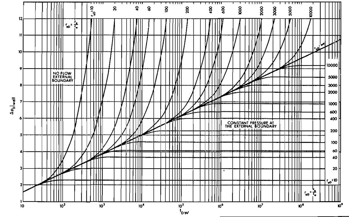
Diagram with values for infinite reservoirs — Pic. 5 Values of Δp_D/well for infinite reservoirs, for finite circular reservoirs with no flow at the external boundary, and for finite circular reservoirs with constant pressure at the external boundary

The equation form of the solution is:

∆ p_{D w} = \frac{2 t_{D w}}{{r_{D e}}^{2}} + \ln (0, 472 r_{D e}) E q . 23

Example 3:

Using the data given in Example 2, find the pressure at the well after the well has been flowing for 1 800 hours.

Solution:

Check for finite or pseudo-steady-state validity:

t_{D θ} = \frac{2, 64 \cdot 10^{- 4} k t}{ϕ \bar{μ} \bar{C} r_{e}^{2}} = \frac{2, 64 \cdot 10^{- 4} (20) (1 800)}{0, 15 (0, 0152) (0, 00061) {(2 000)}^{2}} = 1, 71

Since t_Dθ > 0,25, the well is finite acting.

t_{D w} = \frac{t_{D θ} r_{θ}^{2}}{r_{w}^{2}} = 4, 271 \cdot 10^{7} (> 100)

r_{D θ} = \frac{r_{θ}}{r_{w}} = \frac{2 000}{0, 4} = 5 000

∆ p_{D w} = \frac{2 t_{D w}}{r_{D θ}^{2}} + \ln (0, 472 r_{D θ}) = \frac{2 (4, 271 \cdot 10^{7})}{{(5000)}^{2}} + \ln (0, 472 (5 000)) = 3, 417 + 7, 766

Δp_Dw = 11,183

For Example 2, q_D = 0,0259:

p_{w}^{2} = p_{l}^{2} (1 - q_{D} ∆ p_{D w}) = {(2 000)}^{2} (1 - 0, 0259 (11, 183))

p_{w}^{2} = 2, 841 \cdot 10^{6} p_{w} = 1 686 p s i a

Case 3

If a wen is producing from a reservoir with constant pressure at the outer boundary, that is, in the steady-state condition, the solution to the diffusivity equation is:

∆ p_{D} = \ln r_{D e} . E q . 24

In this case the fixed pressure used in the definition of Δp_D is p_e rather than p_i, where p_e is the constant pressure at the outer boundary. Substituting the definitions of the dimensionless variables will result in Equation 6 presented earlier for steady-state flow.

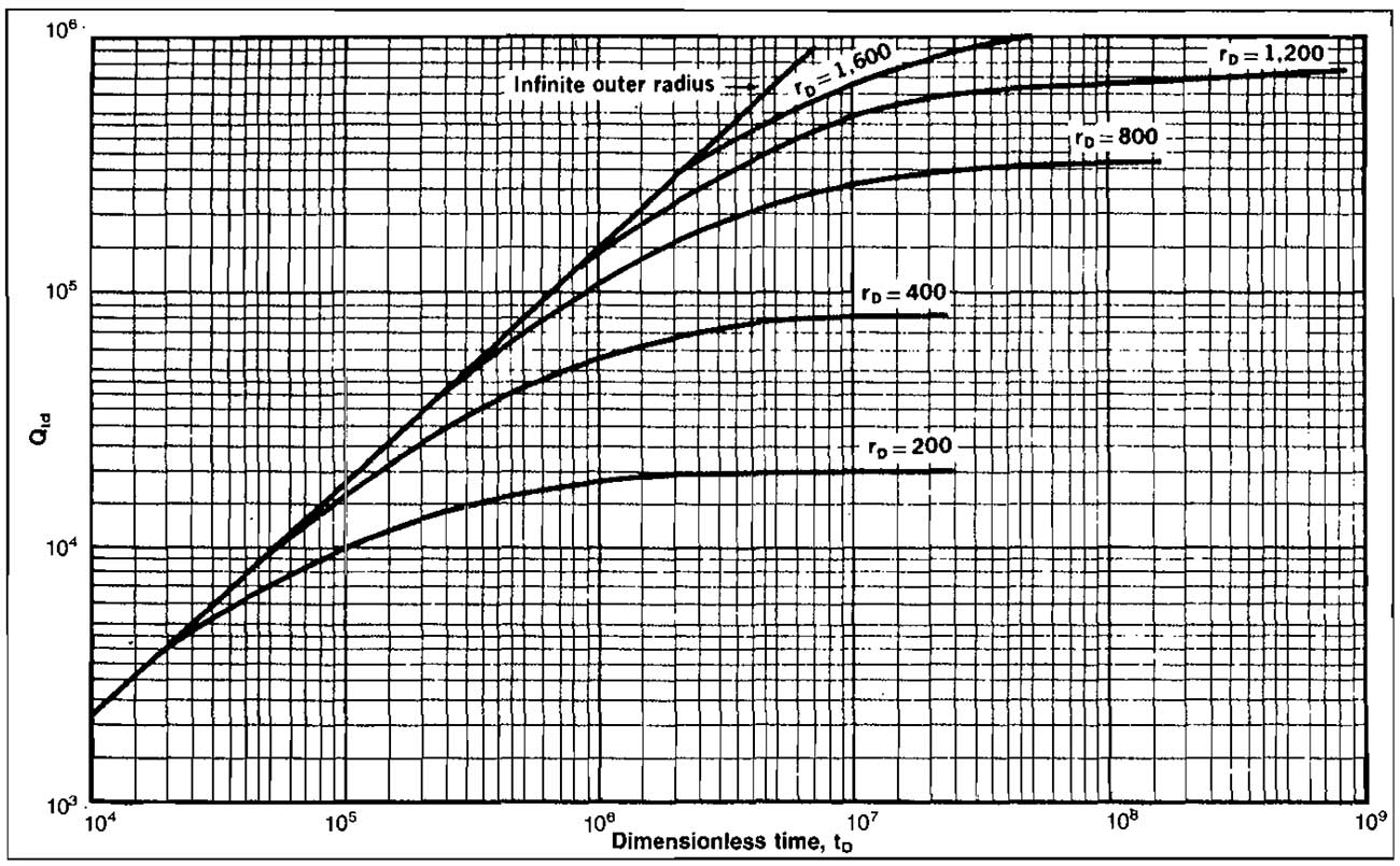
Case 4

The constant pressure solution to the diffusivity equation can be expressed as a function of a dimensionless cumulative production, Q_tD. Q_tD is defined as:

Q_{t D} = \frac{G_{p} \bar{Z} T}{0, 111 ϕ h r_{w}^{2} C (p_{i}^{2} - p_{w}^{2})}, E q . 25

where:

G_p – is the cumulative gas produced in Mscf.

Values of Q_tD as a function of dimensionless time and radius have been presented both graphically and in table form. Pictures 6 and 7 show values of Q_tD versus t_D.

Diagram: constant pressure — Pic. 6 Constant pressure functions

Diagram: constant pressure system — Pic. 7 Constant pressure functions

Noncircular Reservoirs

All of the previous equations were based on a single well draining a circular reservoir, which is rarely ever the actual case. The pressure behavior depends on the shape of the reservoir and the location of the well relative to the boundaries. The time to reach stabilized or pseudo-steady-state flow also depends on these factors.

The previous equations have been modified by Dietz as follows. If the well is still infinite-acting:

∆ p_{D} = 0, 5 [\ln (\frac{A t_{D A}}{r_{w}^{2}}) + . 809], E q . 26

∆ p_{D} = 0, 5 [\ln (\frac{A}{r_{w}^{2} C_{A}}) + . 809] + 2 π t_{DA} . E q . 27

Calculation of t_DA is based on the drainage area and is defined as:

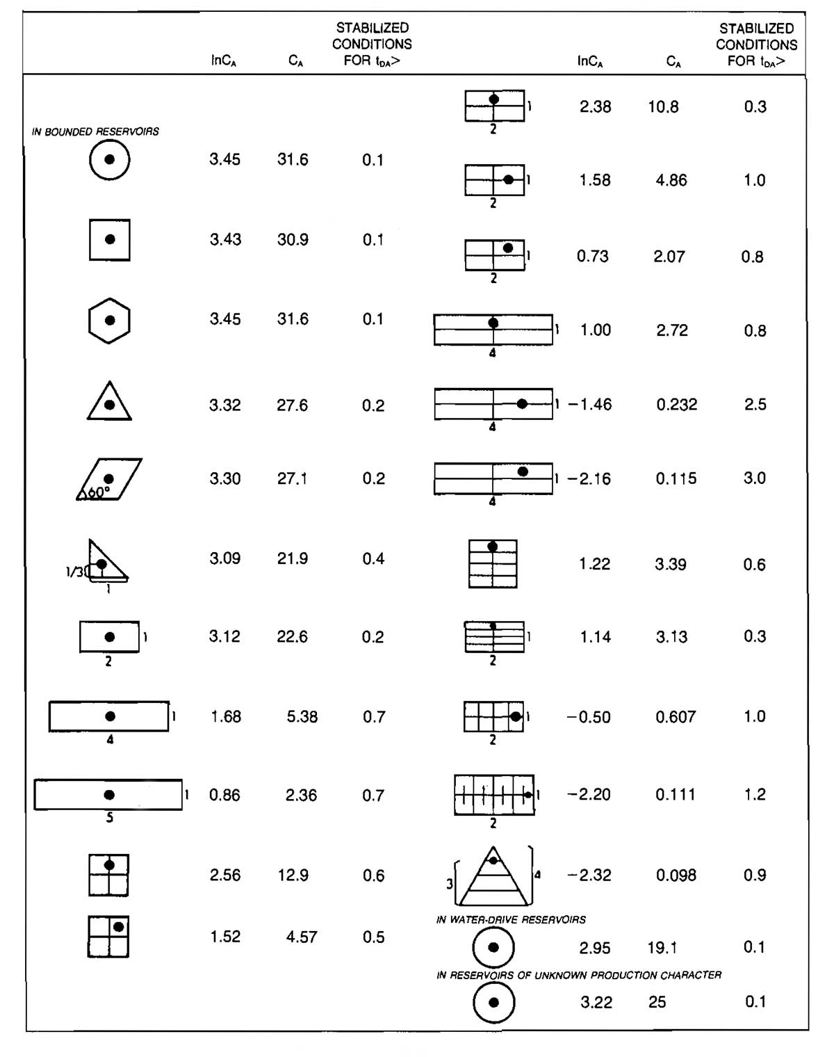
t_{D A} = \frac{2, 64 \cdot 10^{- 4} k t}{ϕ \bar{μ} \bar{C} A} . E q . 28

The shape factor C_A, as well as the value of t_DA required to reach pseudo-steady-state flow can be obtained from Table 2.

Example 3 (a):

Rework Example 3 if the well is located in the center of a rectangular shaped (1·4) drainage area containing 220 acres. (9,58·10⁶ft²).

Solution:

Check for pseudo-steady-state:

t_{D A} = \frac{2, 64 \cdot 10^{- 4} (20) (1 800)}{0, 15 (0, 0152) (0, 00061) (9, 58 \cdot 10^{6})} = 0, 71

Since t_DA > 0,7, the well is in pseudo-steady-state flow. From Table 2, C_A = 5,38 and:

∆ p_{D} = 0, 5 [(\ln \frac{9, 58 \cdot 10^{6}}{{(0, 4)}^{2}) (5, 38)}) + . 809] + 2 π (0, 71)

Δp_D = 8,517+4,461 = 12,978

p_{w}^{2} = p_{i}^{2} (1 - q_{D} ∆ p_{D}) = {(2 000)}^{2} (1 - 0, 0259 (12, 978))

p_{w}^{2} = 2, 655 \cdot 10^{6} p_{w} = 1 630 p s i a

Rock Permeability

All of the equations for reservoir gas flow contain rock and fluid properties that must be known in order to be applied. The fluid properties were presented in Best and Most Widely Methods to Perform Necessary Calculations with a Gas“Methods to Made Calculation of a Gas Producing System”. The only rock property involved in the equations is permeability. In many cases the flow equations will be used to determine permeability by measuring pressures and flow rates. This will be discussed in detail in a subsequent section.

A brief review of the behavior of effective or relative permeability when more than one fluid is present in the rock is given. In most dry gas reservoirs only gas will be flowing even though connate water will be present. In this case the permeability to gas will remain fairly constant over the life of the reservoir. If liquid condensation occurs in the reservoir the permeability to gas will decrease. Condensation of water vapor can also occur near the wellbore in some cases, which will also reduce the permeability to gas in this zone.

The absolute permeability of a rock is defined as a measure of the rock’s ability to transmit a fluid when it is completely saturated with the flowing fluid. The effective permeability to a particular fluid is a measure of the ability of the rock to transmit that fluid in the presence of other fluids. The effective permeability to gas must be used in all of the flow equations presented earlier.

Permeability data are frequently presented as relative permeability. This is the ratio of effective to absolute permeability and therefore varies from zero to one.

Picture 8 presents typical oil and gas relative permeability as a function of liquid saturation. Similar data can be developed for any reservoir and fluid system by core analysis.

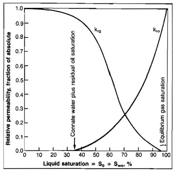
This picture illustrates that the ability of the gas to flow is not seriously impaired until liquid saturation builds up to the point at which liquid begins to flow, about 35 % in this case. It can also be seen that there is a gas saturation below which gas will not flow. This is the equilibrium or critical gas saturation and cannot be recovered.

Well Deliverability or Capacity

The stabilized flow capacity or deliverability of a gas well is required for planning the operation of any gas field. The flow capacity must be determined for different back pressures or flowing bottom-hole pressures at any time in the life of the reservoir and the change of flow capacity with average reservoir pressure change must be considered. The flow equations developed earlier are used in deliverability testing with some of the unknown parameters being evaluated empirically from well tests.

The most common method for determining gas well deliverability is called multipoint testing, in which a well is produced at several different rates (usually four) and from measured flow rates and well pressures, an inflow performance equation can be evaluated. There are basically two types of tests that can be conducted: the flow-after-flow test and the isochronal test. The isochronal test has been modified for very tight wells, but the modification cannot be theoretically justified.

The theory behind the tests is based on the pseudo-steady-state flow equation, Equation 11. Equation 11 may be written as follows:

{\bar{p}}_{R}^{2} - {p_{w f}}^{2} = A q_{s c} + B {q_{s c}}^{2} E q . 11

where:

$A = \frac{1 422 T \bar{μ} \bar{Z}}{k h} (\ln (\frac{. 472 r_{e}}{r_{w}}) + S),$
and;
$A = \frac{1 422 T \bar{μ} \bar{Z}}{k h} D .$

For wells not located in the center of a circular drainage area, the A term is defined as:

A = \frac{1 422 T \bar{μ} \bar{Z}}{k h} [0, 5 \ln (2, 246 A / r_{w}^{2} C_{A}) + S]

where C_A is obtained from Table 2.

It is sometimes convenient to establish a relationship between the two parameters that indicate the degree of turbulence occurring in a gas reservoir. These parameters are the velocity coefficient and the Turbulence Coefficient D. Equation 7 can be written for pseudo-steady-state flow as:

{\bar{p}}_{R}^{2} - {p_{w f}}^{2} = \frac{1 422 T \bar{μ} \bar{Z}}{k h} (\ln \frac{. 472 r_{e}}{r_{w}} + S) q_{s c} + \frac{3, 161 \cdot 10^{- 12} γ_{g} \bar{Z} T β}{r_{w} h^{2}} {q_{s c}}^{2} E q . 29

This form of the equation includes the assumption that r_e≫r_w. Equating the terms multiplying

${q_{s c}}^{2}$

in Equations 11 and 29 yields:

B = \frac{1 422 T \bar{μ} \bar{Z}}{k h} D = \frac{3, 161 \cdot 10^{- 12} γ_{g} \bar{Z} T}{r_{w} h^{2}} β

or:

D = \frac{2, 22 \cdot 10^{- 15} γ_{g} k}{\bar{μ} h r_{w}} β

Expressing β in terms of permeability from Equation 8, the above expression becomes:

D = \frac{5, 18 \cdot 10^{- 5} γ_{g}}{\bar{μ} h r_{w} k^{0, 2}} E q . 30

Equation 11 can also be written in the form:

q_{s c} = C {({\bar{p}}_{R}^{2} - {p_{w f}}^{2})}^{2} . E q . 31

For wells in which turbulence is important the value of n approaches 0,5, while for wells in which turbulence is negligible, n approaches 1,0. In most cases the value of n obtained from well tests will fall between 0,5 and 1,0.

If values for the flow coefficient C and exponent n can be determined, the flow rate corresponding to any value of p_wf can be calculated and an inflow performance curve can be constructed. A parameter commonly used to characterize or compare gas wells is the flow rate that would occur if p_wf could be brought to zero. This is called Absolute Open Flow Potential, or AOF.

Examination of Equation 31 reveals that a plot of:

∆ (p^{2}) = {\bar{p}}_{R}^{2} - {p_{w f}}^{2}

versus q_sc on log-log scales should result in a straight line having a slope of 1/n. At a value of Δ(p²) equal to one, C = q_sc. This is made evident by taking the log of both sides of Equation 31.

\log ({\bar{p}}_{R}^{2} - {p_{w f}}^{2}) = \frac{1}{n} \log q_{s c} - \frac{1}{n} \log C

Once a value of n has been determined from the plot, the value of C can be calculated by using data from one of the tests that falls on the line. That is:

C = \frac{q_{s c}}{{({\bar{p}}_{R}^{2} - {p_{w f}}^{2})}^{n}} .

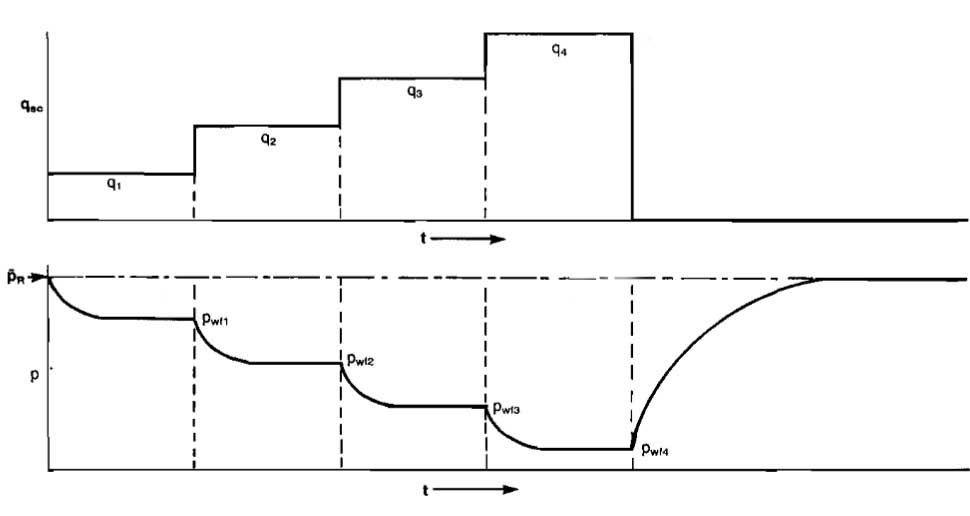
Flow-After-Flow Tests. A flow-after-flow test starts from a shut-in condition. The well is opened on a particular choke size and is not disturbed until the flow rate and p_wf stabilize. This may require a considerable amount of time, depending on the permeability of the reservoir. A well is usually considered to be stabilized if the pressure does not change over a 15-minute interval. Once stabilization is reached, q_sc and p_wf are measured, the rate is changed, and the procedure repeated for several flow rates, usually four. The behavior of flow rate and pressure with time is illustrated in Picture 9 for q_sc increasing in sequence.

Pressure diagrams and test-flow rate — Pic. 9 Conventional test-flow rate and pressure diagrams

The tests may also be run in the reverse sequence. A plot of typical flow-after-flow data is shown in Picture 10.

Diagram: deliverability — Pic. 10 Deliverabilily test plot

Example 4:

A flow-atter-flow test was performed on a well located in a low pressure reservoir in which the permeability was high. Using the following test data, determine:

The values of n and C for the deliverability equation.
The AOF.
The flow rate for p_wf = 160 psia.

Test	q_sc, Mscfd	p_wf, psia	$({\bar{p}}_{R}^{2} - {p_{w f}}^{2}) \cdot 10^{- 3}$
	0	$201 ({\bar{p}}_{R})$	$40, 4 ({\bar{p}}_{R}^{2})$
1	2 730	196	1,985
2	3 970	195	2,376
3	4 440	193	3,152
4	5 550	190	4,301

A plot of q_sc versus Δ(p²) is shown in Picture 11. From the plot it is apparent that tests 1 and 4 lie on the straight line and can thus be used to determine n.

n = \frac{\log q_{1} - \log q_{4}}{\log ∆ {(p^{2})}_{t} - \log ∆ {(p^{2})}_{4}}

n = \frac{\log (2 730) - \log (5 550)}{\log (1, 985 \cdot 10^{3}) - \log {(4, 301 \cdot 10^{3})}^{0, 92}} = 2, 52 \frac{M s c f d}{p s i a^{1, 84}} .

Therefore, the deliverability equation is:

$q_{s c} = 2, 52 {({\bar{p}}_{R}^{2} - {p_{w f}}^{2})}^{0, 92};$
For p_wf = 0, q_sc = 2,52(201²-0²)^.92 = 43,579 Mscfd;
For p_wf = 160 psia, q_sc = 2,52(201²-160²)^.92 = 17,300 Mscfd.

A plot such as Picture 11 may be used directly to obtain the AOF and the well’s inflow performance without calculating values for C and n.

Example of a plot (AOF) — Pic. 11 q_sc versus Δ(p²) plot

The AOF is determined by entering the ordinate at

${\bar{p}}_{R}^{2}$

and reading the AOF as 43,6 MMscfd. An inflow rate at any value of p_wf can be obtained by entering the ordinate at the appropriate value of

$∆ p^{2} = {\bar{p}}_{R}^{2} - {p_{w f}}^{2}$

and reading the rate from the abscissa.

Isochronal Testing. The isochronal, or equal time, test is based on the theory that at equal flow times the same volume of reservoir is affected regardless of flow rate. The isochronal testing method, as introduced by Cullender’ in 1955, has been modified to require even shorter testing times. The modified isochronal test is described in the next section.

The isochronal test was proposed as a means of determining deliverability in tight wells that require a long period of time to reach stabilization. At least one stabilized point is still required to evaluate the coefficient C in Equation 30. The procedure for conducting an isochronal test is:

Starting at a shut-in condition, open the well on a particular choke size for a period of time. Measure q_sc and p_wf at specific time periods for this choke size.
Shut the well in until the pressure returns to
${\bar{p}}_{R} .$
Open the well on a larger choke size and measure q_sc and p_wf at the same flowing time intervals as in Step 1. The total flow periods do not have to be of equal length but they usually are.
Shut the well in until the pressure returns to
${\bar{p}}_{R} .$
Repeat for several choke sizes, usually four.
On the last choke size, allow the well to flow until a stabilized condition is reached. This may require several hours or even days, but only one rate has to be flowed for the long period as compared to all the rates for flow-after-flow testing.

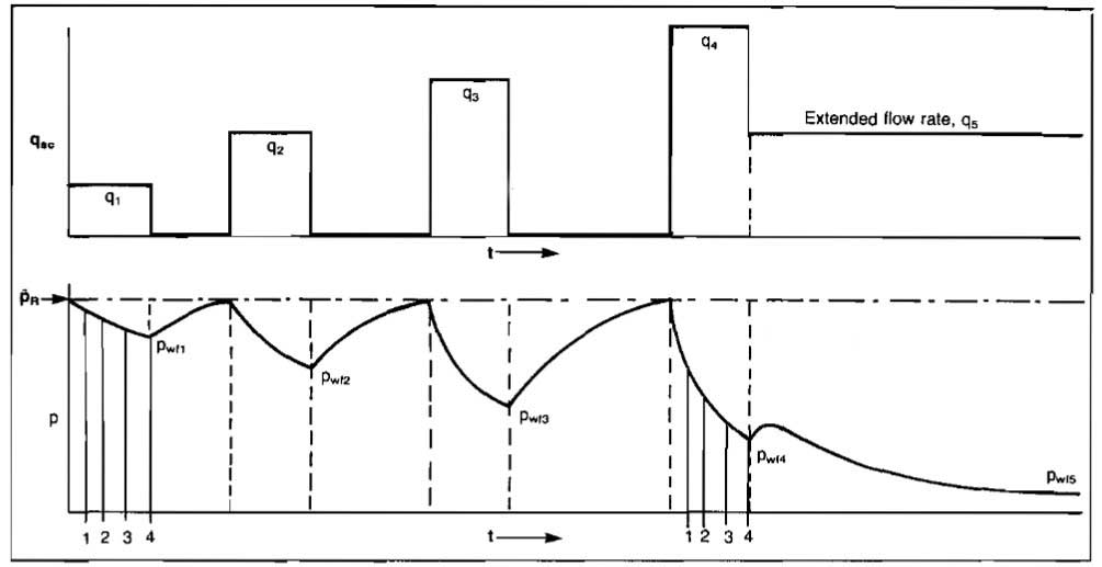
The behavior of the flow rate and pressure with time is illustrated in Picture 12 for increasing flow rates. The reverse order could also be used.

The test is analyzed by plotting

${\bar{p}}_{R}^{2} - {p_{w f}}^{2}$

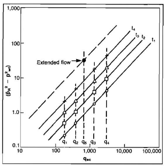
versus q_sc on log-log paper for each flow time at which the data were measured. This will produce one straight line for each flow time, the slopes of which will be equal. The slope allows determination of the exponent n, while the flow coefficient C can be determined using the stabilized or extended flow rate. A plot of typical isochronal flow data is shown in Picture 13.

Typical isochronal flow data — Pic. 13 Isochronal test data

Example 5:

An isochronal test was conducted on a well located in a reservoir that had an average pressure of 1 952 psia. The well was flowed on four choke sizes, and the flow rate and flowing bottom-hole pressure were measured at 3 hr and 6 hr for each choke size. An extended test was conducted for a period of 72 hr at a rate of 6,0 MMscfd, at which time p_wf was measured at 1 151 psia. Using the preceding data, find the following:

Stabilized deliverability equation.
AOF.
Generate an inflow performance curve.

Solution:

	t = 3 hr		t = 6 hr
q_sc, Mscfd	p_wf	${\bar{p}}_{R}^{2} - {p_{w f}}^{2} \cdot 10^{- 3}$	p_wf	${\bar{p}}_{R}^{2} - {p_{w f}}^{2} \cdot 10^{- 3}$
2 600	1 793	597	1 761	709
3 300	1 757	724	1 657	1 064
5 000	1 623	1 177	1 510	1 530
6 300	1 505	1 545	1 320	2 066
6 000	Extended flow, t = 72 hr	1 545	1 320	2 485

1 The slopes of both the 3 hr and 6 hr lines are apparently equal (Pic. 14). Using the first and last points on the 6 hr test to calculate n gives:

n = \frac{\log q_{1} - \log q_{4}}{\log ∆ {(p^{2})}_{1} - \log ∆ {(p^{2})}_{4}} = \frac{\log (2 600) - \log (6 300)}{\log (709) - \log (2 068)} = 0, 83

Diagram: test plot — Pic. 14 Plot of Δp² versus q_sc-isochronal test

Using the extended flow test to calculate C:

C = \frac{q_{s c}}{{({\bar{p}}_{R}^{2} - {p_{w f}}^{2})}^{n}} = \frac{6 000}{{(2 485 \cdot 10^{3})}^{0, 83}} = 0, 0295 .

Therefore, the deliverability equation for q_sc in Mscfd is:

q_{s c} = 0, 0295 {({\bar{p}}_{R}^{2} - {p_{w f}}^{2})}^{0, 83}

2 To calculate AOF, set p_wf = 0:

q_sc = 0,0295(1 952²-0)^0,83 = 8 551 Mscfd

3 In order to generate an inflow performance curve, pick several values of p_wf and calculate the corresponding q_sc.

p_wf, psia	q_sc, Mscfd
1 952	0
1 800	1 768
1 400	4 695
1 000	6 642
600	7 875
200	8 477
0	8 551

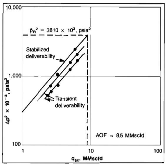
The inflow performance curve is plotted in Picture 15.

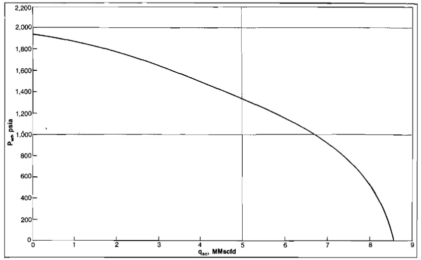
Diagram: the inflow performance curve — Pic. 15 Inflow performance curve, Example 5

If the log-log plot is used to determine the absolute open flow or the inflow performance, the line drawn through the stabilized test must be used.

Modified Isochronal Testing. The modified isochronal testing procedure was introduced so that even less flowing time is required for the well test. The procedure is very similar to the isochronal test, except that the shut-in period between each flow rate is not long enough to allow the well to return to the initial average reservoir pressure. In the modified method the well is shut-in for the same length of time that it was allowed to flow for each choke size. During this time the static well pressure will rebuild to some value, p_ws, which will be lower after each flow period. The flow rate-pressure behavior with time is shown in Picture 16. An extended flow period is still required to evaluate. the flow coefficient C.

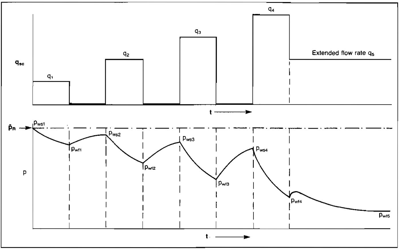
The flow rate-pressure behavior — Pic. 16 Modified isochronal test

The analysis is the same as the regular isochronal test, with the exception that:

∆ (p^{2}) = {p_{w s i}}^{2} - {p_{w f i}}^{2}

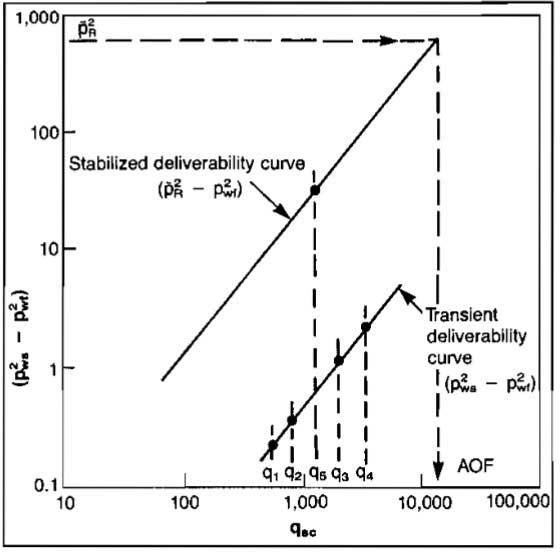
is plotted versus q_sc to obtain a value for n. The value of C is calculated using the initial static or average reservoir pressure and the extended test values for p_wf and q_sc. Picture 17 illustrates a plot of typical modified isochronal test data.

Typical modified isochronal test data — Pic. 17 Modified isochronai test

Jones, Blount and Glaze Method. The method of plotting test data which was proposed by Jones, et al., can be applied to gas well testing to determine real or present time inflow performance relationships. The analysis procedure allows determination of turbulence or non-Darcy effects on completion efficiency irrespective of skin effect and laminar flow, The procedure also evaluates the laminar flow coefficient A, and if k_gh is known, an estimate of skin effect can be made, The data required are either two or more stabilized flow tests or two or more Isochronal flow tests. At least one stabilized flow test is required to obtain a stabilized value of the laminar coefficient A. No transient tests are required-to evaluate the completion efficiency if this method is applied. Jones, et al., also suggested methods to estimate the improvement in inflow performance which would result from reperforating a well to lenglhen the completion interval and presented guidelines to determine if the turbulent effects were excessive. Equation 11 can be divided through by q_sc and written as:

\frac{{\bar{p}}_{R}^{2} - {p_{w f}}^{2}}{q_{s c}} = A + B q_{s c}, E q . 11

where:

A and B are the laminar and turbulent coefficients respectively and are defined in Equation 11.

From Equation 11 it is apparent that a plot of

({\bar{p}}_{R}^{2} - {p_{w f}}^{2}) / q_{s c}

versus q_sc on cartesian coordinates will yield a line that has a slope of B and an intercept of A = Δ(p²)/q_sc as q_sc approaches zero. These plots apply to both linear and radial flow, but the definitions of A and B would depend on the type of flow.

Equation 11 can be solved for flow rate to yield:

q_{s c} = \frac{- A + {[A^{2} + 4 B ({\bar{p}}_{R}^{2} - p_{w f}^{2})]}^{0, 5}}{2 B} E q . 32

In order to have some qualitative measure of the importance of the turbulent contribution to the total drawdown, Jones, et al., suggested comparison of the value of A calculated at the AOF of the well (A^′) to the stabilized value of A. The value of A^′ can be calculated from:

A^′ = A+B(AOF)

where:

A O F = \frac{- A + {[A^{2} + 4 B {\bar{p}}_{R}^{2}]}^{0, 5}}{2 B} . E q . 32 (a)

Jones, et al., suggested that if the ratio of A^′ to A was greater than 2 or 3, then it is likely that some restriction in the completion exists. They also suggested that the formation thickness h used in the definition of B could be replaced by the length of the completed zone h_p, since most of the turbulent pressure drop occurs very near the wellbore. The effect of changing completion zone length on B and therefore on inflow performance can be estimated from:

B_{2} = B_{1} {(\frac{h_{p 1}}{h_{p 2}})}^{2}

where:

B₂ = turbulence multiplier after recomplection;
B₁ = turbulence multiplier before completion;
h_p2 = new completion length, and;
h_p1 = old completion length.

It will be shown in a subsequent section that the improvement in the B term can also be estimated from:

B₂ = B₁(N₁/N₂)²

where:

N – is the total number of effective perforations.

Example 5 (a)

A four-paint test was conducted on a gas well that had a perforated zone of 20 ft. Static reservoir pressure is 5 250 psia, Using the Jones, et al., method, determine:

A and B.
AOF.
Ratio of A^′/A.
New AOF if the perforated interval is increased to 30 ft.

Test Data
Test No.	q_sc, Mscfd	p_wf, psia
1	9 300	5 130
2	6 000	5 190
3	5 200	5 203
4	3 300	5 225

Solution:

Test No.	q_sc, Mscfd	$({\bar{p}}_{R}^{2} - {p_{w f}}^{2}) / q_{s c}, p s i a^{2} / M s c f d$
1	9 300	133,9
2	6 000	104,4
3	5 200	94,5
4	3 300	79,4

From a plot of this data, Picture 17 (a), it is found that:
- A = 48 psia²/Mscfd;
- B = 9,24·10^-3 psia²/Mscfd²;
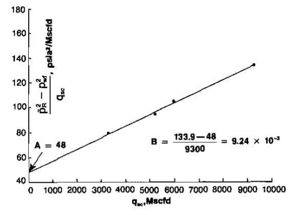
Pic. 17 (a) Jones et al., Method
$A O F = \frac{- 48 + {[48^{2} + 4 (9, 24 \cdot 10^{- 3}) {(5 250)}^{2}]}^{0, 5}}{2 (9, 24 \cdot 10^{- 3})}$
AOF = 52,080 Mscfd.
A^′ = 48+9,24·10^-3(52 080) = 529
A^′/A = 529/48 = 11;
B₂ = B₁(h_p1/h_p2)²
B₂ = 9,24·10^-3(20/30)² = 4,1·10^-3
$A O F_{2} = \frac{- 48 + {[48^{2} + 4 (4, 1 \cdot 10^{- 3}) {(5 250)}^{2}]}^{0, 5}}{2 (4, 1 \cdot 10^{- 3})}$
AOF₂ = 76,340 Mscfd.

The value of A^′ calculated in the previous example indicates a large degree of turbulence. The effect of increasing the perforated interval on the AOF is substantial. Further implications of the effects of well completion efficiency will be discussed in the section on Well Completion Effects.

Laminar Inertia Turbulence (LIT) Analysis

All of the previously described methods for predicting gas well deliverability or inflow performance require at least one test conducted for a period long enough to reach stabilization. Equation 21 can be used to calculate the approximate time to stabilization as follows:

t_{S} = \frac{950 ϕ \bar{μ} \bar{C} {r_{e}}^{2}}{k} = \frac{380 ϕ \bar{μ} \bar{C} A}{k} E q . 33

This can be a very long period of time in low permeability reservoirs, especially if a well is draining a large area.

Several methods have been proposed for obtaining a deliverability equation without a stabilized test. Essentially the only difference in these methods is the method used to obtain the coefficients A and B in Equation 11. A method presented by Brar and Aziz’ will be described in this section.

The pseudo-steady-state equation for gas flow is:

∆ (p^{2}) = {\bar{p}}_{R}^{2} - {p_{w f}}^{2} = A q_{s c} + B {q_{s c}}^{2} E q . 11

For unsteady-state flow, A varies with time and will be written as A_i. The equations can be written in terms of common logs rather than natural logs. For pseudo-steady-state:

∆ (p^{2}) = 2 m [\log (\frac{. 472 r_{e}}{r_{w}}) + \frac{S}{2, 303}] q_{s c} + 0, 869 m D {q_{s c}}^{2} E q . 34

where:

m = \frac{1 637 T \bar{μ} \bar{Z}}{k h} E q . 35

For transient flow:

∆ (p^{2}) = m [\log (\frac{k t}{ϕ \bar{μ} \bar{C} {r_{w}}^{2}}) - 3, 23 + . 869 S] q_{s c} + 0, 869 m D {q_{s c}}^{2} E q . 36

Comparing Equations 34 and 36 to Equation 11 implies that:

A = 2 m [\log (\frac{0, 472 r_{e}}{r_{w}}) + \frac{S}{2, 303}] E q . 37

A_{r} = m [\log (\frac{k t}{ϕ \bar{μ} \bar{C} {r_{w}}^{2}}) - 3, 23 + 0, 869 S] E q . 38

and:

B = 0,869md Eq. 39

The object of the analysis is to be able to determine the values of A and B for stabilized flow, then Equation 11 can be used to calculate inflow performance. The skin factor S, the turbulence coefficient D, and the permeability k can also be determined.

Equation 36 may be written as:

\frac{∆ (P^{2})}{q_{s c}} = A_{r} + B q_{s c}

where A_r and B are defined in Equations 38 and 39 respectively. The value of A_r will increase with time until stabilized flow is reached. A plot of Δ(p²)/q_sc versus q_sc on cartesian coordinates will result in a series of straight, parallel lines having slopes equal to B and intercepts A_r equal Δ(p²)/q_sc for each flow time. The slopes and intercepts can also be determined using least squares analysis. Equation 38 can be expressed as:

A_{r} = m [\log \frac{k}{ϕ \bar{μ} \bar{C} {r_{w}}^{2}} - 3, 23 + . 869 S] + m \log t

Therefore a plot of A_t versus t on the semi-log scales will result in a straight line having a slope equal to m and an intercept at t = 1 hr (log 1 = 0) equal to A_tI. The procedure for analyzing an Isochronal test is:

Determine A_t and B from transient tests for several flow times using plots of Equation 36 or least squares.
Plot A_r versus t on semi-log scales to determine m and A_tI.
Using the value of m, calculate k from Equation 35.
Solve Equation 38 for S using the values of m, k, and A_rI.
Calculate a stabilized value for A using Equation 37.
Using the value of B from Step 1, calculate D using Equation 39.
Calculate the stabilized well performance from Equation 11 using the stabilized values for A and B.

The method of least squares may be used to determine A_t and B from N transient flow tests.

A_{r} = \frac{Σ \frac{∆ (p^{2})}{q} Σ q^{2} - Σ ∆ (p^{2}) Σ q}{N Σ q^{2} - Σ q Σ q} E q . 40

B = \frac{N Σ ∆ (p^{2}) - Σ \frac{∆ (p^{2})}{q} Σ q}{N Σ q^{2} - Σ q Σ q} E q . 41

Values for A_r and B will be obtained for each time at which p_wf was measured. The value of B should be constant, and Brar and Aziz suggest using the value of B obtained from the longest flow test as the representative value.

Values for A_t and B can also be obtained by plotting the data as illustrated in Picture 17 (a). In this case a different line would be obtained for each time at which pressures were measured, resulting in a value of A_t which will increase with increasing time.

Example 6:

A modified isochronal test was conducted using four different flow rates, and the flowing bottom-hole pressure was measured at periods of 1, 2, 4, 6, and 8 hours. The test data are tabulated below.

h = 12 ft.
r_w = 0,23 ft.
ϕ = 0,23.
T = 582 °R.
r_θ = 2 000 ft.
${\bar{p}}_{R}$
= 922,6 psia.
$\bar{μ}$
= 0,0116 cp.
$\bar{Z}$
= 0,972.
$\bar{C}$
= 0,00109 psia^-1.

	p_ws
	922,6	921,9	919,9	917,6
t	p_wf
t	q = 0,4746	q = 0,8797	q = 1,2716	q = 1,6589
1,0	900,1	863,0	798,9	676,3
2,0	897,1	853,9	769,9	662,2
4,0	892,2	833,0	754,9	642,0
6,0	890,1	827,9	732,8	635,2
8,0	888,1	825,1	727,3	629,3

Use the test data to determine k, S, D, and the stabilized deliverability equation.

Solution:

Table 3 may be constructed to conveniently calculate the vaiue for A_t and B. To further illustrate the procedure, some of the entries for t = 2 hr are calculated.

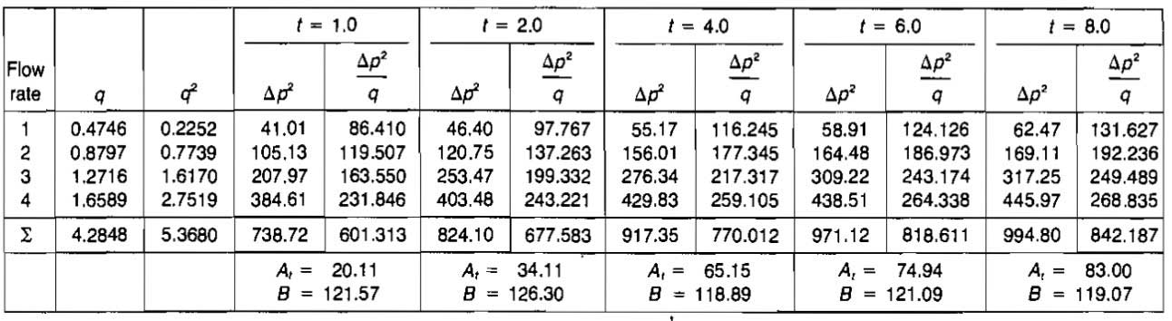
For q_sc = 0,4746 MMscfd:

∆ (p^{2}) = {p_{w s}}^{2} - {p_{w f}}^{2} = {(922, 6)}^{2} - {(897, 1)}^{2} = 46, 402 p s i a^{2}

\frac{∆ (p^{2})}{q} = \frac{46 402}{0, 4746} = 97, 767 \frac{p s i a^{2}}{M M s c f d} = 97, 767 \frac{M p s i a^{2}}{M M s c f d}

A_{t} = \frac{(677, 583) (5, 368) - (824, 1) (4, 2848)}{4 (5, 368) - (4, 2848) (4, 2848)} = 34, 11 \frac{M p s i a^{2}}{M M s c f d}

B = \frac{4 (824, 1) - (677, 583) (4, 2848)}{4 (5, 368) - {(4, 2848)}^{2}} = 126, 30 \frac{M p s i a^{2}}{M M s c f d^{2}}

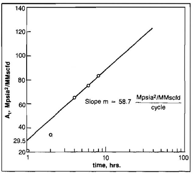
The values calculated for A_t are plotted versus t on semi-log paper in Picture 18. The slope of the line is m = 58,7 Mpsia²/MMscfd/cycle obtained by drawing a straight line through the last three points. The intercept at t = 1 hr can be read from the graph as 29,5 Mpsia²/MMscfd.

From Equation 35:

k = \frac{1 637 T \bar{μ} \bar{Z}}{m h} = \frac{1 637 (528) (0, 0116) (0, 972)}{(58, 7) (12)}

k = 13,8 md

Solving Equation 38 for S, using the value of A_t at t = 1 hr:

S = [\frac{A_{(1)}}{m} - \log \frac{k (1)}{ϕ \bar{μ} \bar{C} {r_{w}}^{2}} + 3, 23] (\frac{1}{. 869})

S = [\frac{29, 5}{58, 7} - \log (\frac{13, 8 (1)}{. 23 (0, 0116) (0, 00109) {(0, 23)}^{2}}) + 3, 23] (1, 151)

S = -4,22

To obtain the turbulence coefficient, solve Equation 39 for D:

D = \frac{B}{0, 869 m} = \frac{119, 07}{0, 869 (58, 7)} = 2, 23 M M s c f d^{- 1}

Equation 34 may now be used to calculate A:

A = 2 (58, 7) [\log (\frac{. 472 (2 000)}{0, 23}) + \frac{(- 4, 22)}{2, 303}]

A = 209 \frac{p s i a^{2}}{M s c f d}

The value chosen for B is 119,07 Mpsia²/MMscfd² = 0,1191 psia²/Mscfd².

The stabilized fiow equation for determining inflow performance is then:

{\bar{p}}_{R}^{2} - {p_{w f}}^{2} = 209 q_{s c} + 0, 1191 {q_{s c}}^{2}

for p in psia and q_sc in Mscfd.

Equation 29 may be solved for q_sc to obtain:

q_{s c} = \frac{- A + {(A^{2} + 4 B ({\bar{p}}_{R}^{2} - {p_{w f}}^{2}))}^{0, 5}}{2 B} E q . 42

For A = 209 and B = 0,1191:

q_{s c} = \frac{- 209 + (43 681 + 0, 4764 {({\bar{p}}_{R}^{2} - {p_{w f}}^{2}))}^{0, 5}}{0, 2382}

The AOF for this well can be calculated using p_wf = 0 as:

A O F = \frac{- 209 + (43 681 + 0, 4764 {(922, 6)}^{2})^{0, 5}}{0, 2382}

AOF = 1 936 Mscfd

Factors Affecting Inflow Performance. Once a well has been tested and the deliverability or inflow performance equation established, it is sometimes desirable to be able to predict how changes in certain parameters will affect the inflow performance. These changes may be the result of reservoir depletion or time, or they may result from well workovers.

The effects of various’ changes can be estimated by reference to Equations 31 and 10.

q_{s c} = C {({\bar{p}}_{R}^{2} - {p_{w f}}^{2})}^{2} E q . 31

Comparing this with Equation 10, it can be seen that the effect of turbulence, Dq_sc are included in the exponent n, and the coefficient C contains several parameters subject to change.

C = \frac{703 \cdot 10^{- 6} k h}{T \bar{μ} \bar{Z} [\ln (\frac{. 472 r_{e}}{r_{w}}) + S]} E q . 43

The possible causes of changes in each parameter are discussed and modifications of C are suggested.

The only factor that has an appreciable effect on permeability to gas, k is liquid saturation in the reservoir. As pressure declines from depletion, the remaining gas expands to keep S_g constant, unless retrograde condensation occurs or water influx is present. For dry gas reservoirs, the change in k with time can be considered negligible.
In most cases the value of formation thickness, h can be considered constant. A possible exception is if the completion interval is changed by perforating a longer section. It is likely that the well would be re-tested at this time.
Reservoir temperature, T will remain constant, except for possible small changes around the wellbore.
Gas Viscosity and Compressibility Factor,
$\bar{μ}$
and
$\bar{Z}$
are the parameters that are subject to the greatest change as
${\bar{p}}_{R}$
changes. The best method to handle these changes will be discussed in a later section on pseudo-pressure analysis. An approximation of the effect of changes in
${\bar{p}}_{R}$
on C can be made by modifying C as follows:
$\frac{C_{1}}{C_{2}} = \frac{{(\bar{μ} \bar{Z})}_{2}}{{(\bar{μ} \bar{Z})}_{1}} . E q . 44$
The drainage radius, r_e depends on the well spacing and can be considered constant once stabilized flow is reached.
The wellbore radius, r_w can be considered to remain constant. It is possible that the effective wellbore radius can be changed by stimulation, but this can be accounted for in the skin factor.
The skin factor, S can be changed by fracturing or acidizing a well. The well should be retested at this time to re-evaluate both C and n.

Example 7:

Generate future inflow performance curves for the well in Example 5 at values of average reservoir pressure of 1 500 psia and 1 000 psia. The following additional data are known:

γ_g = 0,70;
Reservoir temperature = 200 °F.

Solution:

In order to correct for the changes in viscosity and compressibility factor, these will be calculated based on

${\bar{p}}_{R} :$

${\bar{p}}_{R}$	μ	Z	μZ	C
1 952	0,0156	0,86	0,0134	0,0295
1 500	0,0148	0,88	0,0130	0,0304
1 000	0,0134	0,91	0,0122	0,0324

For
${\bar{p}}_{R} = 1 500 p s i a, q_{s c} = 0, 0304 {(1 500^{2} - {p_{w f}}^{2})}^{0, 83} .$
For
${\bar{p}}_{R} = 1 000 p s i a, q_{s c} = 0, 0324 {(1 000^{2} - {p_{w f}}^{2})}^{0, 83} .$

	q_sc, Mscfd
p_wf, psia	${\bar{p}}_{R} = 1 500 p s i a$	${\bar{p}}_{R} = 1 000 p s i a$
1 500	0	–
1 200	2 437	–
1 000	3 494	0
600	4 924	2 136
300	5 501	2 861
0	5 691	3 094

The data are plotted in Picture 19.

Diagram: performance curve — Pic. 19 Inflow performance curve, Example 7

In many cases it will be impossible or impractical to obtain multi-rate tests at the same value of

${\bar{p}}_{R}$

That is, flow rates and either flowing wellhead or bottomhole pressures may be obtained over a long time span during the producing life of the well. These periodic tests are frequently required by regulatory agencies. If it is assumed that neither C nor n has changed during the time span, then Equation 31 will apply for all values of

${\bar{p}}_{R}$

and p_wf. That is, a plot of the data as illustrated in Picture 10 should result in a straight line even though different values of

${\bar{p}}_{R}$

were used to calculate Δ(p²). A value of n can be obtained from the slope and a value for C can be calculated using one of the test points which falls on the line. The resulting equation would then be valid as long as both C and n remain constant. A similar approach could be used for the Jones, Blount and Glaze method if it is assumed that both A and B in Equation 11 remain constant.

Transient Testing

Methods have been presented for determining the stabilized deliverability or inflow performance of a gas well for use in planning equipment purchases and other field development procedures.

Much useful reservoir information can be obtained from various types of unsteady-state or transient gas well tests. Information that can be obtained from transient tests includes permeability k, skin factor S, turbulence coefficient D, and average reservoir pressure,

${\bar{p}}_{R}$

. If a test is continued into the pseudo-steady-state flow regime, an estimate of reservoir size can be made. This is usually called a reservoir limit test.

The most common transient tests are drawdown tests and buildup tests. Essentially the same information can be obtained from each. The choice of which type of test to run depends on well and field conditions.

Any test that involves a change in flow rate is analyzed based on the principle of superposition. This principle, as it applies to well testing, is briefly described.

Principle of Superposition. The superposition principle in effect states that if a pressure disturbance is created in a reservoir, the disturbance continues to travel through the reservoir even though the source of the disturbance may change or cease. This means that in order to determine the pressure at a location as a function of time, all of the pressure disturbance effects must be added.

Superposition in Time. When the flow rate is changed in a well, the pressure disturbance caused by the previous flow rate continues to affect the reservoir. As an analogy, when the source of a noise is stopped, the sound waves already emitted do not stop. Consider the case in which a well is produced at some rate q₁ for a time t₁. The rate is then changed to q₂ and flow is continued. If the pressure is desired at some time t₂, the effect of both rates must be considered. The flow rate and pressure behavior are illustrated in Picture 20.

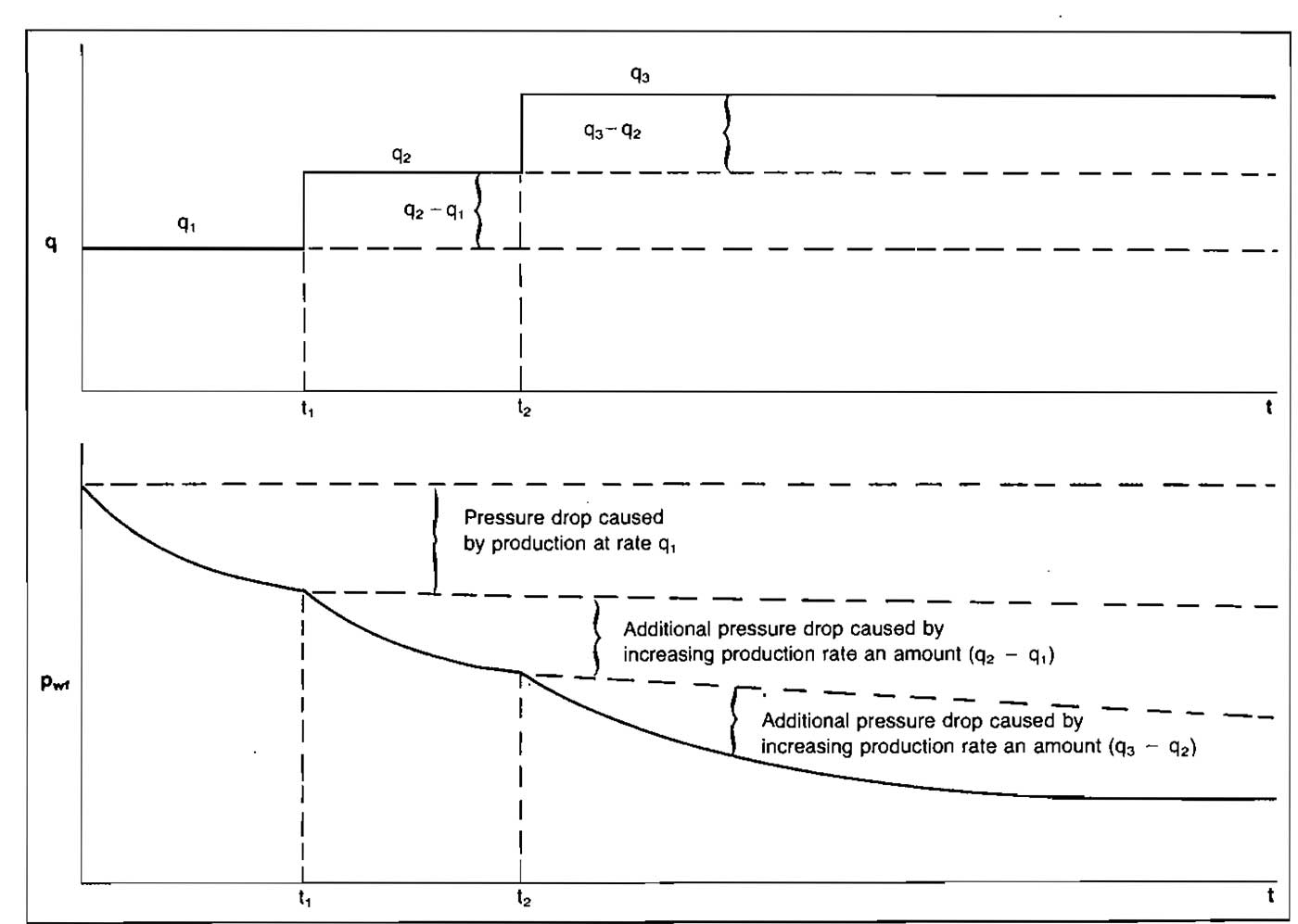
Diagram: pressure behavior — Pic. 20 Superposition

Adding the effect of the two rates flowing for their respective times gives:

{p_{i}}^{2} - {p_{w f}}^{2} = {p_{i}}^{2} q_{D 1} ∆ p_{D 1} + {p_{i}}^{2} q_{D 2} ∆ p_{D 2} E q . 45

where:

q_{D 1} = \frac{1 422 T \bar{Z} \bar{μ}}{k h {p_{i}}^{2}} q_{1}, E q . 46

q_{D 2} = \frac{1 422 T \bar{Z} \bar{μ}}{k h {p_{i}}^{2}} (q_{2} - q_{1}), E q . 47

Δp_D1 is based on total flowing time, t₁+t₂, Δp_D2 is based on flowing time t-t₁.

Superposition in Space. When more than one well is producing in a reservoir, the effects of both pressure disturbances must be added to calculate the total pressure effect at any point in the reservoir. This of course requires evaluation of pressure at points other than the well. This is the basis for interference testing involving two or more wells. Superposition in time and space can be applied simultaneously.

Pressure Drawdown Testing. Several important reservoir parameters can be determined by flowing a well at a constant rate and measuring flowing wellbore pressure as a function of time. This is called drawdown testing and it can utilize information obtained in both the transient and pseudo-steady-state flow regimes. If the flow extends to pseudo-steady-state, the test is referred to as a Reservoir Limit Test and can be used to estimate the reservoir pore volume. Both single rate and two rate tests are utilized, depending on the information required. Some of the reservoir parameters which may be obtained from drawdown testing are flow capacity kh, skin factor S, and turbulence coefficient D.

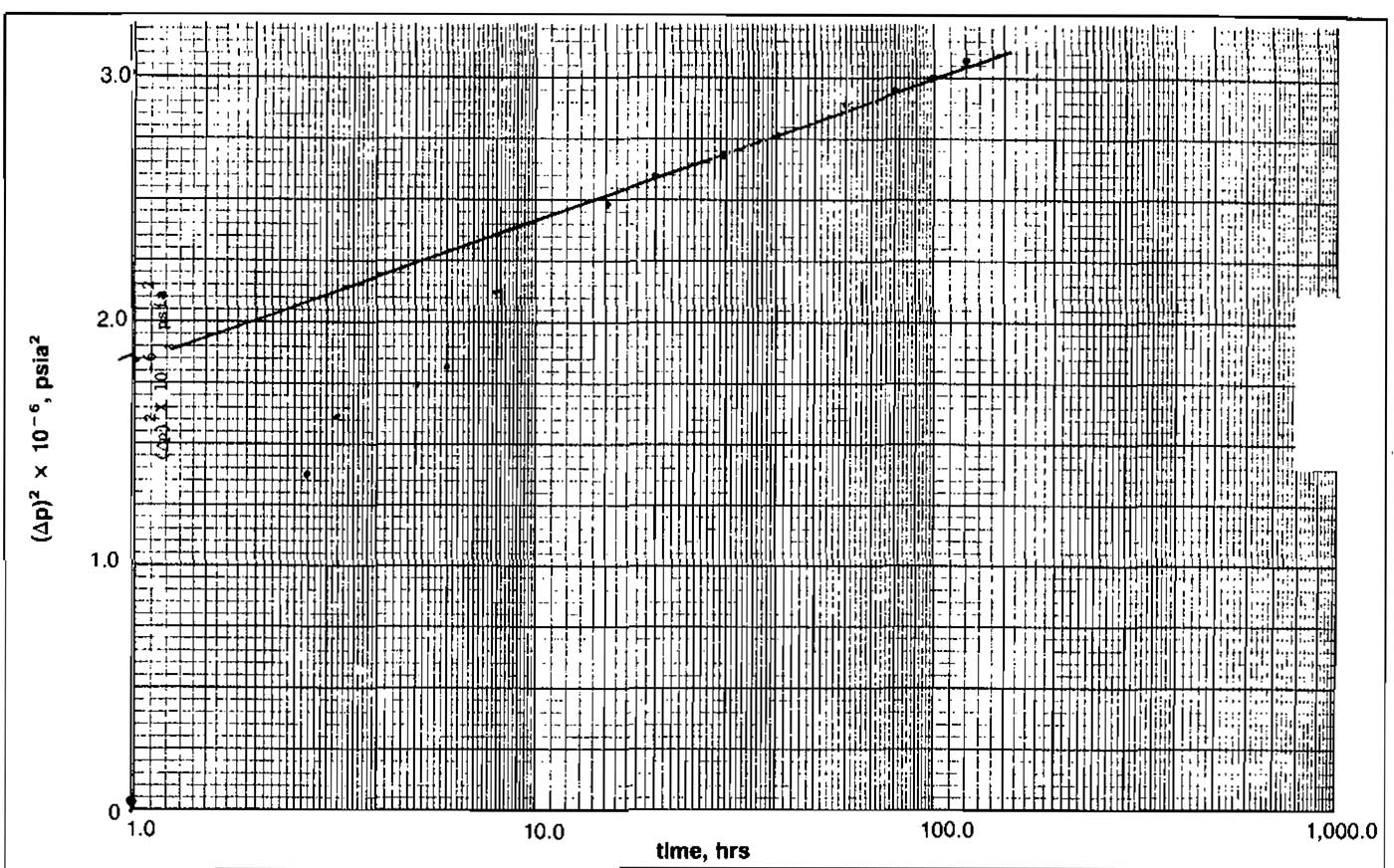
A drawdown test begins from a shut-in condition and a constant flow rate is maintained while pressure is measured constantly. The early time pressure data will be affected by wellbore storage and is usually used only to determine the beginning of the transient flow period. This can be identified as the beginning of the straight line segment of the plot of (Δp²) versus time.

The equation for transient flow, Equation 20, may be written including formation damage and turbulence effects as:

Δp_D = 0,5(ln t_D+.809)+S^′ Eq. 48

where:

S^′ = S+Dq_sc.
S = actual well damage or improvement, such as clay swelling, or fractures, and may be positive or negative.
D = turbulence coefficient, which will always be positive.

In terms of real variables and common logs, Equation 48 becomes:

{p_{i}}^{2} - {p_{w f}}^{2} = \frac{1 637 q_{s c} T \bar{μ} \bar{Z}}{k h} [\log t + \log \frac{k}{ϕ \bar{μ} \bar{C} {r_{w}}^{2}} - 3, 23 + 0, 869 S^{'}], E q . 49

where k is in millidarcys.

From this form of the equation it can be seen that a plot of Δ(p²) vs. log t will give a straight line of slope m, where:

m = \frac{1 637 q_{s c} T \bar{μ} \bar{Z}}{k h} E q . 50

from which kh can be calculated. To obtain S^′, let t = 1 hr (log 1 = 0), then:

{p_{i}}^{2} - {p_{1}}^{2}_{h r} = m [\log \frac{k}{ϕ \bar{μ} \bar{C} {r_{w}}^{2}} - 3, 23 + 0, 869 S^{'}], E q . 51

where p_1hr is obtained from an extrapolation of the linear segment of the plot. Solving for S^′ in Equation 51 gives:

S^{'} = 1, 151 [\frac{{p_{i}}^{2} - {p_{1}}^{2}_{h r}}{m} - \log \frac{k}{ϕ \bar{μ} \bar{C} {r_{w}}^{2}} + 3, 23] . E q . 52

Since S^′ is rate dependent, two single rate drawdown tests may be concducted to determine S and D. That is, from the two tests:

{S^{'}}_{1} = S + D q_{1}

{S^{'}}_{2} = S + D q_{2} .

The removable pressure drop due to actual damage can be calculated from:

Δ(p²)_S = 0,869mS, Eq. 53

and the rate dependent pressure drop from:

Δ(p²)_D = 0,869mDq_sc, Eq. 54

An estimate of the beginning and end of the transient flow period can be obtained from the dimensionless time once an estimate of k is obtained from the analysis. The approximate range of dimensionless time for transient flow is:

0,03≤t_De≤0,25.

If the segment chosen for obtaining the straight line slope did not fall within this range, the data should be re-examined.

A problem also results in determining at what pressure to calculate the fluid properties since the pressure is constantly changing during the test. The properties required are viscosity, Z-factor and isothermal compressibility. These properties be calculated at an average pressure defined as:

\bar{p} = {[(p_{i}^{2} + p_{w f}^{2}) / 2]}^{0, 5},

where p_wf is the lowest flowing bottomhole pressure used in the analysis.

Example 8:

The following data apply to a well on which a drawdown test was conducted. Use the data to calculate k and S^′.

p_i = 3 732 psia.
ϕ = 0,10.
$\bar{μ}$
= 0,021 cp.
$\bar{C}$
= 2,2·10^-4psi^-1.
T = 673 °R.
r_w = 0,29 ft.
γ_g = 0,68.
h = 20 ft.
r_θ = 2 640 ft.
$\bar{Z}$
= 0,85.
q_sc = 5,65 MMscfd.

t, hr	p_wf, psia	$∆ (p^{2}) = p_{i}^{2} - {p_{w f}}^{2} \cdot 10^{- 6}, p s i a^{2}$
1,60	3 729	0,022
2,67	3 546	1,354
3,20	3 509	1,615
5,07	3 491	1,741
6,13	3 481	1,810
8,00	3 433	2,142
15,20	3 388	2,449
20,00	3 366	2,598
30,13	3 354	2,679
40,00	3 342	2,759
60,27	3 323	2,885
80,00	3 315	2,939
100,27	3 306	2,998
120,53	3 295	3,071

From the graph of Δ(p²) versus log t (Pic. 21) the slope is:

m = \frac{3 \cdot 10^{6} - 2, 42 \cdot 10^{6}}{\log 100 - \log 10} = 5, 8 \cdot 10^{5} p s i a^{2} / c y c l e,

and:

k h = \frac{1 637 q_{s c} T \bar{μ} \bar{Z}}{m} = \frac{1 637 (5 650) (673) (0, 021) (0, 85)}{5, 8 \cdot 10^{5}},

kh = 192 md-ft,

k = \frac{192}{20} = 9, 6 m d .

Test of drawdown pressure — Pic. 21 Pressure drawdown test, Example 8

To obtain p_thr, extend the line to t = 1 hr and read:

Δ(p²) = 1,84·10⁶ psia²

S^{'} = 1, 151 [\frac{1, 84 \cdot 10^{6}}{0, 58 \cdot 10^{6}} - \log (\frac{9, 6}{0, 1 (0, 021) (2, 2 \cdot 10^{- 4}) {(0, 29)}^{2}}) + 3, 23]

S^′ = 1,151(3,172-8,393+3,23) = -2,29

To estimate the extra pressure drop due to skin at the test flow rate:

∆ {(p^{2})}_{S^{'}} = 0, 869 m S^{'} = 0, 869 (5, 8 \cdot 10^{5}) (- 2, 29)

∆ {(p^{2})}_{S^{'}} = - 1, 154 \cdot 10^{6} p s i a^{2}

Two-Rate Tests. The two-rate test consists of flowing the well at a rate q₁ for a period t and then changing the rate to q₂. The pressure and rate behavior are illustrated in Picture 22.

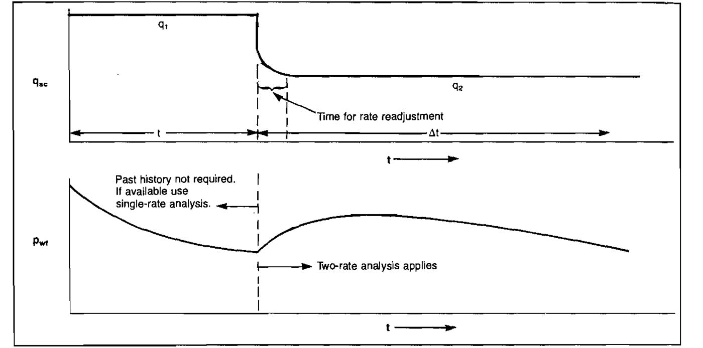
The pressure and rate behavior — Pic. 22 Two-rate test-flow rate and pressure diagrams

By applying superposition in time it can be shown that a plot of:

∆ (p^{2}) v e r s u s \log (\frac{t + ∆ t}{∆ t}) + \frac{q_{2}}{q_{1}} \log ∆ t

on cartesian coordinates will yield a straight line of slope:

m = \frac{1 637 q_{1} T \bar{μ} \bar{Z}}{k h} .

If the data from the first flow period are analyzed to obtain

$S_{1}^{'}$

a value for

$S_{2}^{'}$

can be calculated from:

q_{1} S_{1}^{'} - q_{2} S_{2}^{'} = \frac{q_{1} ∆ {(p^{2})}_{1} - ∆ {(p^{2})}_{0}}{0, 869 m} - \frac{(q_{1} - q_{2})}{0, 869} [\log \frac{k}{ϕ \bar{μ} \bar{c} r_{w} 2} - 3, 23], E q . 55

where:

Δ(p²)₁ is read at Δt = 1;
Δ(p²)₀ is read at Δt = 0.

Reservoir Limit Test. If a drawdown test is allowed to flow until the reservoir boundary is felt (pseudo-steady-state), the pressure behavior is governed by Equation 23 for circular reservoirs or by Equation 27 for noncircular reservoirs. By rearranging Equation 23 and putting it in terms of real variables, it can be shown that a plot of Δ(p²) versus time on cartesian coordinates will yield a straight line of slope m. This can be used to estimate the in place volume of gas in the reservoir, G.

G = \frac{2, 348 q_{s c} T}{μ C m}

where G is the gas volume in MMscf.

Pressure Buildup Testing. A pressure buildup test is the simplest test that can be run, on a gas well. If the effects of wellbore storage can be determined, much useful information can be obtained. This information includes permeability, k, apparent skin factor, S^′, and average reservoir pressure,

${\bar{p}}_{R} .$

The test consists of flowing the well at a constant rate q_sc, for a period of time t, shutting the well in (at Δt = 0), and measuring wellbore pressure increase with shut-in time Δt.

The test was developed by Horner, and his method of analysis is generally considered best. Other methods include those of Miller, Dyes, and Hutchinson and Muskat. The method was extended to allow determination of average reservoir pressure for bounded reservoirs by Matthews, Brons, and Hazebroek (MBH).

The theory behind the buildup test comes from superposition in time. In order to represent the shut-in condition, an injection rate of -q_sc beginning at Δt = 0 is superposed on the flow rate q_sc that began at time t = 0. Writing Equation 48 for both q_sc and -q_sc and adding the expressions results in:

p_{i}^{2} - p_{w s}^{2} = \frac{1 637 q_{s c} T \bar{μ} \bar{Z}}{k h} \log \frac{t + ∆ t}{∆ t} . E q . 56

From this expression it can be seen that a plot of

${p_{w s}}^{2}$

versus log((t+Δt/Δt)) will result in a straight line of slope – m, where:

m = \frac{1 637 q_{s c} T \bar{μ} \bar{Z}}{k h}, E q . 50

from which kh or k can be determined.

Extrapolation of the line to an infinite shut in time Δt, or (t+Δt)/Δt = 1, results in a value for

$p_{i}^{2}$

for an infinite reservoir. For bounded reservoir this value is labeled p^*2 and can be used to obtain

${\bar{p}}_{R}$

, as described later.

The apparent skin factor can be determined by assuming that (t/(t+Δt)) ≈ 1 at Δt = 1 hr and using the following equation:

S^{d} = 1, 151 [\frac{p_{1 h r}^{2} - {p_{w f}}^{2}}{m} - \log \frac{k}{ϕ \bar{μ} \bar{C} r_{w}^{2}} + 3, 23], E q . 576

where:

p_1hr is read from the extrapolated straight line at Δt = I hr and;
p_wf is the flowing wellbore pressure at shut-in (Δt = 0).

The permeability k is in millidarcys in this equation.

The value of

${\bar{p}}_{R}$

for finite or bounded reservoirs may be determined using the MBH method. The value obtained from extrapolating the line to infinite Δt, referred to as p^*, is neither the initial reservoir pressure p_i, nor the average reservoir pressure

${\bar{p}}_{R}$

. It is a pseudo-pressure that will fall between these values.

${\bar{p}}_{R}$

can be obtained from p* by using curves prepared by MBH for various shapes of drainage areas. A relationship between p* and

${\bar{p}}_{R}$

is plotted as a function of dimensionless time based on drainage area, t_DA.

t_{D A} = \frac{2, 64 \cdot 10^{- 4} k t}{ϕ \bar{μ} \bar{C} A} E q . 28

where:

t = producing time before shut-in, hrs, and;
A = drainage area, ft².

The value obtained from the curves for the appropriate t_DA is:

\frac{2, 303 (p^{* 2} - {\bar{p}}_{R}^{2})}{m}, E q . 58

from which a value of

${\bar{p}}_{R}$

can be obtained. An example MBH curve is illustrated in Picture 24. Curves for other conditions are in the appendix.

The fluid properties for buildup analysis should be calculated at an average pressure defined by:

\bar{p} = {[(p^{* 2} + p_{w f}^{2}) / 2]}^{0, 5} .

Example 9:

The well described in Example 8 was flowed at a rate of 5,65 MMscfd for a period of 120,5 hours and then shut-in for a buildup test. The flowing pressure at shut-in was 3 295 psia. Calculate k, S^′, and

${\bar{p}}_{R}$

if the well is producing from the center of a square drainage area containing 22·10⁶sq. ft. The pressure versus time data are tabulated below.

Solution:

Δt, hr	p_ws, psia	$\frac{t + ∆ t}{∆ t}$	p_ws²·10^-6, psia
0	3 295	–	10,86
,53	3 296	228,4	10,86
1,60	3 385	76,3	11,46
2,67	3 547	46,1	12,58
3,73	3 573	33,3	12,77
4,80	3 591	26,1	12,90
5,87	3 605	21,5	13,00
6,93	3 614	18,4	13,06
8,00	3 623	16,1	13,13
9,87	3 634	13,2	13,21
12,00	3 644	11,0	13,28
14,67	3 654	9,2	13,35
18,67	3 664	7,5	13,42
24,53	3 672	5,9	13,48
29,33	3 676	5,1	13,51
35,73	3 684	4,4	13,57
45,87	3 688	3,6	13,60
49,87	3 691	3,4	13,62

The plot of p_ws² versus log((t+Δt)/Δt) is shown in Picture 23.

Diagram: pressure buildup — Pic. 23 Pressure buildup, Example 9

Matthews, Brons, and Hazebroek curves — Pic. 24 MBH curves for well in center of area

The slope may be obtained by taking the change in p_ws² over 2 log cycles.

m = \frac{(13, 92 - 12, 72) \cdot 10^{6}}{\log 100 - \log 1} = 6 \cdot 10^{5} p s i a^{2} / c y c l e

k h = \frac{1 637 q_{s c} T \bar{μ} \bar{Z}}{m} = \frac{1 637 (5 650) (673) (0, 021) (0, 85)}{6 \cdot 10^{5}}

k h = 185 m d - f t k = \frac{185}{20} = 9, 3 m d

At:

∆ t = 1 h r, \frac{t + ∆ t}{∆ t} = 121, 5, {p_{1 h r}}^{2} = 12, 69 \cdot 10^{6}

S^{'} = 1, 151 [\frac{12, 69 \cdot 10^{6} - 3 295^{2}}{6 \cdot 10^{5}} - . . . \log (\frac{9, 3}{(0, 1) (0, 021) (2, 2 \cdot 10^{- 4}) {(0, 29)}^{2}}) + 3, 23]

S^{'} = 1, 151 (3, 055 - 8, 379 + 3, 23) = - 2, 41

The values obtained for k and S^′ agree with those obtained from the drawdown test, Example 8.

In order to estimate

${\bar{p}}_{R}$

, obtain p^*2 from the graph where (t+Δt)/Δt = 1 to be 13,92·10⁶psia². Using the value for k to calculate t_DA gives:

t_{D A} = \frac{2, 64 \cdot 10^{- 4} (9, 3) (120, 5)}{(0, 10) (0, 021) (2, 2 \cdot 10^{- 4}) (22 \cdot 10^{6})} = 0, 029

From Table 2, the well is still in unsteady-state flow if t_DA<0,1, which is the case for this example. Therefore, p^* = p_i = 3 731 psia.

Equation 11 may be used to predict the stabilized performance of a well by utilizing the results of a transient test. However, this requires isolation of the effects of actual formation damage or simulation from those caused by non-Darcy or turbulent flow. That is, S^′ must be broken down into its components S and Dq_sc. If transient test was conducted at only one flow rate, Equation 30 may be used to estimate D, and then S may be calculated from S = S^′-Dq_sc.

Applying this procedure to Example 9 results in:

D = \frac{5, 18 \cdot 10^{- 5} γ_{g}}{\bar{μ} h r_{w} k^{0, 2}} = \frac{5, 18 \cdot 10^{- 5} (. 68)}{. 021 (20) (. 29) {(9, 3)}^{0, 2}}

D = 1,85·10^-4 Mscfd^-1

S = S^′-Dq_sc = -2,41-1,85·10^-4(5 650)

S = -2,41-1,05 = -3,46

Real Gas Pseudo-Pressure Analysis

In deriving the equation for reservoir gas flow in terms of Δ(p²), one step involved evaluation of the integral:

2 \int_{P_{w}}^{P_{e}} \frac{p d p}{μ Z} . E q . 59

Both μ and Z are functions of pressure and therefore should be included in the integration. In order to simplify the derivation it was assumed that μ and Z could be considered constant at reservoir temperature and average pressure in the drainage area, which resulted in

$\bar{μ}$

and

$\bar{Z}$

appearing in all of the flow equations. For fairly low pressure reservoirs (

${\bar{p}}_{R}$

≤2 500 psia) this approach is adequate, but for some pressure ranges the μZ product is far from linear with pressure. A method to more rigorously evaluate the effects of μ and Z was introduced by Al-Hussainy in 1965. He defined the integral in Equation 59 as the real gas pseudo-pressure, m(p).

m (p) = \int_{P_{m}}^{P} 2 \frac{p}{μ Z} d p E q . 60

All of the previously derived equations in this article can be modified to the pseudo-pressure analysis from the p² analysis by replacing the pressure squared terms with the pseudo-pressure terms and eliminating the

$\bar{μ} \bar{Z}$

product from the equation. As an example, Equation 11 becomes:

m ({\bar{p}}_{R}) - m (p_{w}) = \frac{1 422 T q_{s c}}{k h} [\ln (0, 472 r_{e} / r_{w} + S + D q_{s c}], E q . 61

where:

$m ({\bar{p}}_{R})$
is the value of the pseudo-pressure function at the pressure
${\bar{p}}_{R}$
, and;
m(p_w) is the value at pressure p_w.

The definitions of some of the dimensionless variables defined in Table 1 will change if the m(p) approach is used.

q_{D} = \frac{1 422 T q_{s c}}{k h m (p_{i})},

p_{D} = \frac{m (p)}{m (p_{i}) q_{D}},

∆ p_{D} = \frac{m (p_{i}) - m (p)}{m (p_{i}) q_{D}},

t_{D} = \frac{2, 64 \cdot 10^{- 4} k t}{ϕ μ_{i} C_{i} r^{2}},

where C_i and μ_i are evaluated at p_i, T. The m(p) analysis may also be used in deliverability testing. This involves substitution of Δm(p) for Δ(p²) in the procedure to find A_t and B in the LIT analysis.

Use of the m(p) approach requires generation of a table or graph of m(p) versus p for the gas in question at reservoir temperature. This is easily accomplished by numerical integration of Equation 60 when values of μ and Z can be found in Best and Most Widely Methods to Perform Necessary Calculations with a Gas“Methods to Made Calculation of a Gas Producing System”. A computer. program for generating the m(p) versus p values is given in the appendix. An example calculation of m(p) data, as presented by Dake is illustrated.

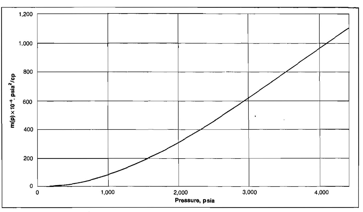
Example 10:

A reservoir existing at a temperature of 200 °F contains a gas having a gravity of 0,85. Generate a relationship between m(p) and p over the pressure range of 4 400 to zero psia.

Solution:

The following table is used to tabulate the data, taking pressure increments of 400 psi for averaging. The results are plotted in Picture 25.

Diagram: pseudopressure — Pic. 25 Real gas pseudopressure, as a function of the actual pressure

Example 11:

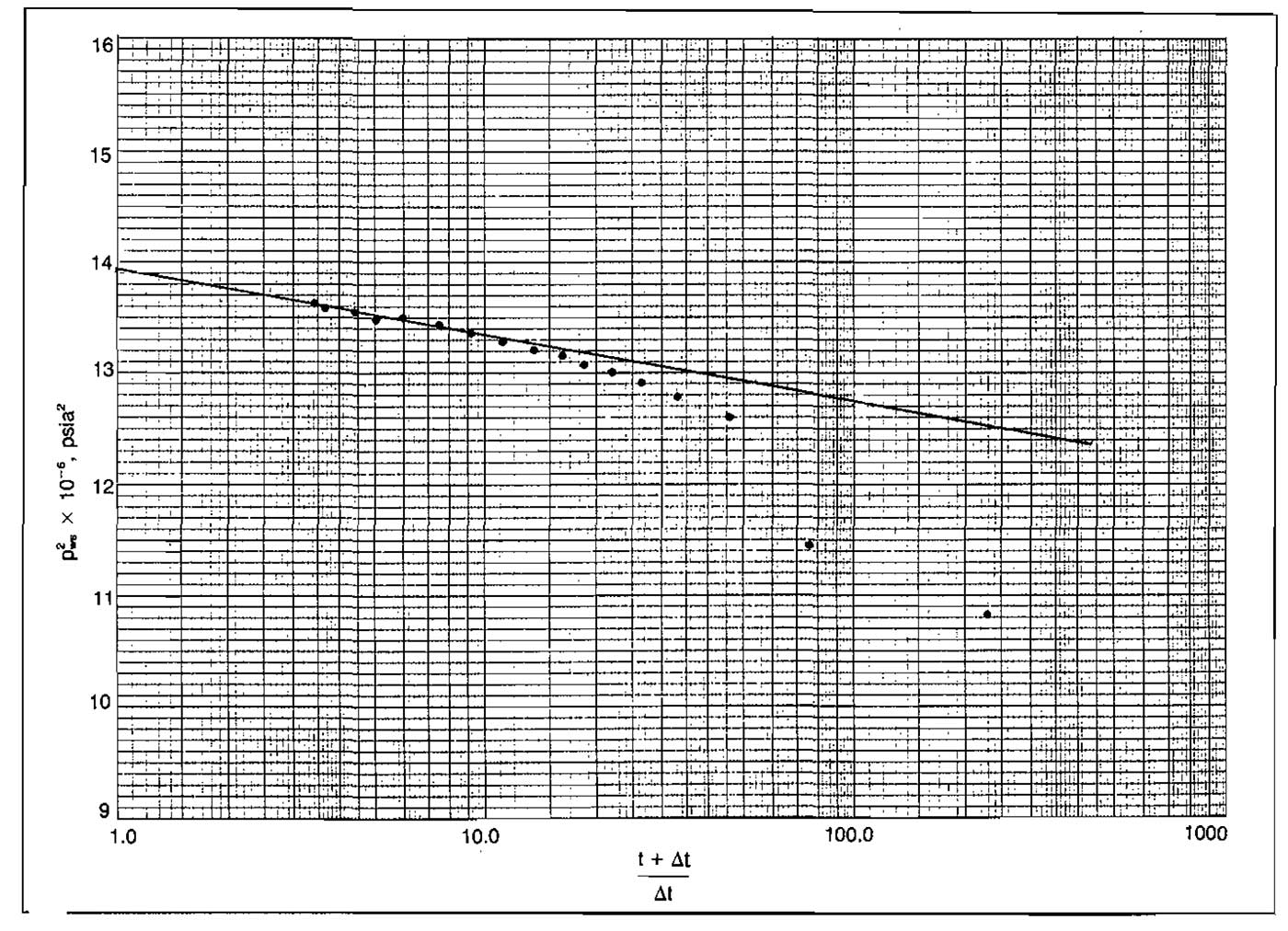
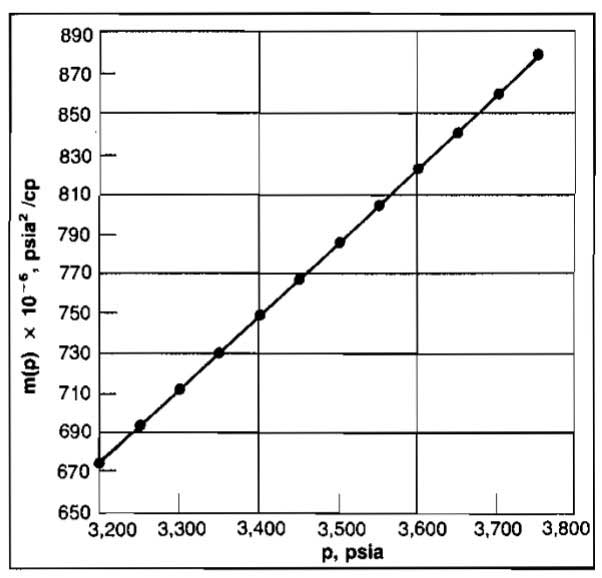
Analyze the buildup test of Example 9 using the pseudo-pressure analysis to obtain k, S^′ and

${\bar{p}}_{R}$

. The relationship between p and m(p) is given in Picture 26.

Diagram with data for "example 11" — Pic. 26 m(p) versus p data, Exampie 3-11.

Solution:

Values for m(p) and (t+Δt)/Δt are calculated and tabulated as follows.

Δt, hrs.	p_ws, psia	formula	m(p)·10^-6, psia²/cp
0,00	3 295	–	709,8
0,53	3 296	228,4	710,1
1,60	3 385	76,3	742,7
2,67	3 547	46,1	802,8
3,73	3 573	33,3	812,6
4,80	3 591	26,1	819,3
5,87	3 605	21,5	824,6
6,93	3 614	18,4	828,0
8,00	3 623	16,1	831,4
9,87	3 634	13,2	835,5
12,00	3 644	11,0	839,3
14,67	3 654	9,2	843,1
18,67	3 664	7,5	846,8
24,53	3 672	5,9	849,9
29,33	3 676	5,1	851,4
35,73	3 684	4,4	854,5
45,87	3 688	3,6	855,9
49,87	3 691	3,4	857,1

A plot of m(p) versus log ((t+Δt)/Δt) is shown in Picture 27.

Graph for example 11 — Pic. 27 Horner build-up plot for Example 11

The slope of the straight line segment is:

m = \frac{(873, 0 - 842, 5) \cdot 10^{6}}{\log 10 - \log 1} = 30, 5 \cdot 10^{6}

k h = \frac{1 637 q_{s c} T}{m} = \frac{1 637 (5 650) (673)}{30, 5 \cdot 10^{6}} = 204 m d - f t

k = \frac{204}{20} = 10, 2 m d

At Δt = 1 hr, m(p_1hr) = 809·10⁶.

S^{'} = 1, 151 [\frac{m (p_{1 h r}) - m (p_{w f})}{m} - \log \frac{k}{ϕ μ_{i} C_{i} {r_{w}}^{2}} + 3, 23]

S^{'} = 1, 151 [\frac{(809, 0 - 709, 8) \cdot 10^{6}}{30, 5 \cdot 10^{6}} - \log . . . \frac{10, 2}{0, 10 (0, 021) (2, 2 \cdot 10^{- 4}) {(0, 29)}^{2}} + 3, 23]

S^′ = -2,2

These values of k and S^′ agree with those obtained in Example 9.

In order to obtain a value for p^* = p_i(t_DA<0,1), read m(p^*) at (t+Δt)/t = 1 to be 873·10⁶. This corresponds to a value of p_i = 3 730 psia, which is equal to the result obtained previously.

It has generally been recommended in the literature that the pseudo-pressure analysis be used in preference to the pressure-squared analysis when p_i = 2 500 psia. The only extra work involved in using the m(p) method is generation of the m(p) versus p data. This task has somehow delayed the acceptance of the m(p) method among field engineers, and many prefer using the more familiar p² analysis. Some advantages of the m(p) method are:

It is more theoretically correct;
It applies for all ranges of pressure;
Iteration to obtain
$\bar{p} = (p_{i} + p_{w f}) / 2$
for evaluating
$\bar{μ} \bar{Z}$
is not necessary, and;
Once m(p) versus p is available, it is simpler to use.

Gas Reserves

All of the flow equations used in the previous sections of this article involved either initial reservoir pressure p_i, or average reservoir pressure

${\bar{p}}_{R}$

. These pressures are functions of the gas in place in a reservoir and must be evaluated at various times in the reservoir life. The flow capacity or deliverability of the wells declines as gas is produced and

${\bar{p}}_{R}$

declines. Therefore, it is necessary to be able to predict

${\bar{p}}_{R}$

versus gas produced G_p.

In order to evaluate a gas reservoir the original gas in place G, must be determined and the gas recoverable at different values of

${\bar{p}}_{R}$

must be calculated. The decline in

${\bar{p}}_{R}$

with G_p can be calculated using the gas laws presented in Best and Most Widely Methods to Perform Necessary Calculations with a Gas“Methods to Made Calculation of a Gas Producing System” for a volumetric reservoir. If the volume occupied by gas changes because of water influx, it must be accounted for in the balance. This section will present methods to determine gas reservoir behavior using volumetric methods and material balance methods.

Reserve Estimates – Volumetric Method

The volumetric method for determining initial gas in place and reserves requires enough geologic data to determine reservoir pore volume and water saturation. Reservoir pressure is also required, but no production history is necessary. It is applied mainly in new fields for rough estimates.

The equation for calculating gas in place is:

G = \frac{43 560 A h ϕ (1 - S_{w})}{B_{g}}, E q . 62

where:

G = gas in place, scf;
A = area of reservoir, acres;
h = average reservoir thickness, ft;
ϕ = porosity;
S_w = water saturation, and;
B_g = gas formation volume factor, ft³/scf.

This equation can be applied at both initial and abandonment conditions in order to calculate the recoverable gas.

Gas produced = Initial gas – Remaining gas

or:

G_{p} = 43 560 A h ϕ (1 - S_{w}) (\frac{1}{B_{g i}} - \frac{1}{B_{g a}}), E q . 63

where B_ga is evaluated at abandonment pressure. Application of the volumetric method assumes that the pore volume occupied by gas is constant. If water influx is occurring, A, h, and S_w will change.

Example 12:

A gas reservoir has the following characteristics. Calculate the gas recovered and the recovery factor at pressures of 1 000 psia and 500 psia.

A = 2 550 acres;
S_w = 20 %;
γ_g = 0,70;
h = 50 ft;
T = 186 °F;
ϕ = 0,20;
p_i = 2 651 psia.

p	Z	B_g
2 651	0,83	0,0057
1 000	0,90	0,0154
500	0,95	0,0346

Solution:

At p = 1 000 psia:

G_{p} = 43 560 (2 550) (50) (0, 2) (1 - 0, 2) \cdot (\frac{1}{0, 0057} - \frac{1}{0, 0154})

G_p = 8,886·10⁸(175,44-64,94) = 9,818·10¹⁰ scf

E_{g} = 1 - \frac{B_{g i}}{B_{g a}} = 1 - \frac{0, 0057}{0, 0154} = 0, 63 = 63 %

At p = 500:

G_{p} = 8, 886 \cdot 10^{8} (\frac{1}{0, 0057} - \frac{1}{0, 0346})

G_p = 8,886·10⁸(175,44-28,90) = 13,02·10¹⁰ scf

E_{g} = 1 - \frac{0, 0057}{0, 0346} = 0, 835 = 83, 5 %

The recovery factors for volumetric gas reservoirs will range from 80 to 90 %. If a strong water drive is present, trapping of residual gas at higher pressures can reduce the recovery factor substantially, to the range of 50 to 80 %.

Reserve Estimates – Material Balance Method

If enough production-pressure history is available for a gas reservoir, the initial gas in place G, the initial reservoir pressure, p_i, and the gas reserves can be calculated without knowing A, h, ϕ or S_w. This is accomplished by forming a mass or mole balance on the gas. That is:

Moles Produced = initial moles in place – remaining moles

in equation form:

n_p = n_i – n. Eq. 64

Applying the gas law, pV = ZnRT gives:

\frac{p_{s c} G_{p}}{T_{s c} Z_{s c}} = \frac{p_{i} V_{i}}{T_{f} Z_{i}} - \frac{p V_{i}}{T_{f} Z}, E q . 65

where:

T_f = formation temperature;
V_i = reservoir gas volume;
p_i = initial reservoir pressure, and;
p = reservoir pressure after producing G_p scf.

The reservoir gas volume can be put in units of scf by use of B_gi. That is:

V_i = GB_gi. Eq. 66

Combining Equations 65 and 66 and solving for p/Z gives:

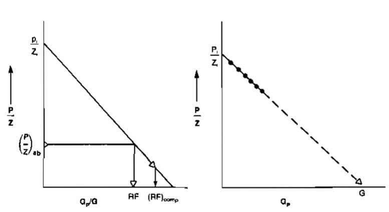
\frac{p}{Z} = \frac{p_{i}}{Z_{i}} - \frac{T_{f} p_{s c}}{T_{s c} B_{g i} G} G_{p} E q . 67

from which it is obvious that a plot of p/Z versus G_p will produce a straight line of slope (T_fp_sc/T_scB_giG) and intercept at G_p = 0 of p_i/Z_i. Thus, both G and p_i can be obtained graphically. Once these values are obtained, a value of gas recovered G_p, can be determined for any pressure. Equation 67 can also be expressed in terms of recovery factor as:

\frac{p}{Z} = \frac{p_{i}}{Z_{i}} (1 - \frac{G_{p}}{G}) . E q . 68

Picture 28 illustrates typical plots of Equations 67 and 68.

Schemes: material balance — Pic. 28 Gas material balance plots

Gas material balance — Pic. 28 (a) Example 13 Solution

Example 13:

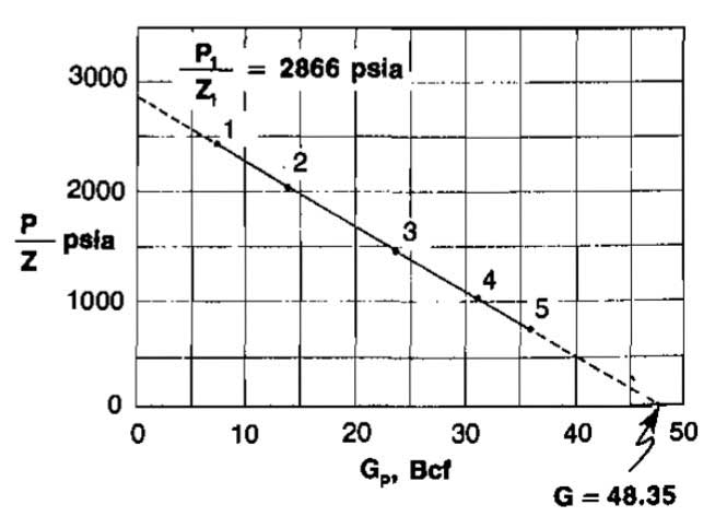
The following production history was obtained from a volumetric gas reservoir. Plotting of p/Z versus G_p revealed that data points 1 and 4 fall on the best straight line through the data. Use these points to find G and p_i/Z_i. Also estimate the gas recovery if the reservoir pressure is drawn down to 300 psia. T_f = 200 F, γ_g = 0,9.

	p, psia	Z	p/Z	G_p, Bcf
1	1 885	0,767	2 458	6,873
2	1 620	0,787	2 058	14,002
3	1 205	0,828	1 455	23,687
4	888	0,866	1 025	31,009
5	645	0,900	717	36,207

Solution:

Using points 1 and 4, calculate the slope:

m = \frac{{(p / Z)}_{1} - {(p / Z)}_{4}}{G_{p 4} - G_{p 1}} = \frac{2 458 - 1 025}{31, 009 - 6, 873} = 59, 37 \frac{p s i a}{B c f}

To find p_i/Z_i, use Equation 67 and data point 1:

\frac{p_{i}}{Z_{i}} = \frac{p}{Z} + m G_{p} = 2 458 + 59, 37 (6, 873) = 2 866 p s i a

B_{g i} = 0, 0283 \frac{T_{f} Z_{i}}{p_{i}} = \frac{0, 0283 (660)}{2 866} = 0, 0065 f t^{3} / s c f

G = \frac{T_{f} p_{s c}}{T_{s c} B_{g i} m} = \frac{p_{i}}{Z_{i} m} = \frac{2 866}{59, 37} = 48, 3 B c f

Recovery at p = 300 psia:

At p = 300 psia, Z = 0,949, p/Z = 316 psia.

G_{p} = (\frac{p_{i}}{Z_{i}} - \frac{p}{Z}) / m = \frac{(2 866 - 316)}{59, 37} = 42, 95 B c f .

The value of p_i can be obtained from p_i/Z_i by trial-and-error. Values of p_i are estimated; Z_i and p_i/Z_i are calculated until a value is determined that gives 2 866 psia.

p_i	Z_i	p_i/Z_i
2 200	.750	2 933
2 100	.752	2 793
2 150	.751	2 863

Linear interpolation between 2 200 and 2 150 gives p_i = 2 151 psia.

The above discussion applies to a reservoir in which the pore volume occupied by gas does not change, If water influx is occurring, V_i will be reduced by water influx as p declines.

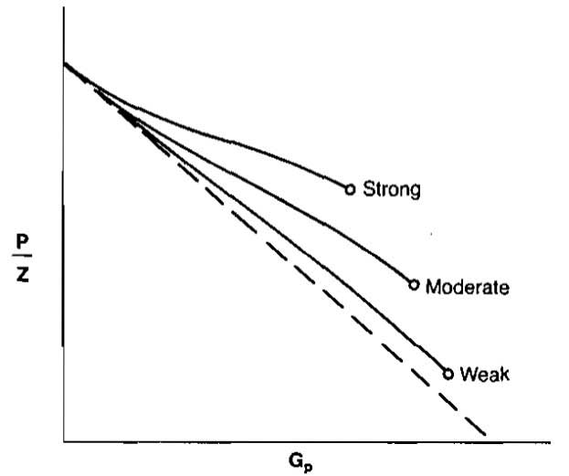
Equation 67 then becomes:

\frac{p}{Z} = (\frac{G B_{g i}}{G B_{g i} - W_{e}}) \frac{p_{i}}{Z_{i}} - \frac{T_{f} p_{s c}}{T_{s c} (G B_{g i} - W_{e})} G_{p} . E q . 69

The slope now includes a quantity that varies with G_p or time. This is the water influx W_e. Therefore, a plot of p/Z versus G_p will no longer be linear but will deviate upward with pressure decline depending on the strength of the water drive. This is illustrated in Picture 29.

Strong, moderate and weak effect of water drive — Pic. 29 Effect of water drive

If water influx is occurring, it can be calculated by using the constant pressure solution to the diffusivity equation, Equation 70. This involves the correct determination of certain water influx parameters. Havlena and Odeh have described a procedure by which the material balance equation can be used to determine if these parameters have been correctly evaluated.

Water influx is a function of time, and can be expressed as:

W_e = CΣΔpQ_tD, Eq. 70

where:

C = water influx constant;
Δp = p_i-p_t;
Q_tD = dimensionless water influx.

The value of Q_tD depends on the ratio of the aquifer volume to the gas reservoir volume and the time that the reservoir has been produced. Values may be obtained from Pictures 6 and 7.

Energy Plots

Many other graphieal methods have been proposed for solving the material balance equation that are useful in detecting the presence of water influx. Equation 67 can be rearranged and using the definition of B_gi = (p_scZ_iT_f)/(p_iT_sc), it can be written as:

\frac{Z_{i} p}{p_{i} Z} = \frac{G B_{g i}}{G B_{g i} - W_{e}} [1 - \frac{G_{p}}{G}] . E q . 71

For W_e = 0, this becomes:

1 - \frac{Z_{i} p}{p_{i} Z} = \frac{G_{p}}{G} . E q . 72

Taking the logarithm of both sides of Equation 72 yields:

\log [1 - \frac{Z_{i} p}{p_{i} Z}] = \log G_{p} - \log G . E q . 73

From Equation 73, it is obvious that a plot of 1 – Z_ip/p_iZ versus G_p on log-log coordinates will yield a straight line with a slope of one (45° angle). An extrapolation to one on the vertical axis (p = 0) yields a value for initial gas in place, G. The graphs obtained from this type of analysis have been referred to as Energy Plots. They have been found to be useful in detecting water influx early in the life of a reservoir. If W_e is not zero, the slope of the plot will be less than one, and will also decrease with time, since W_e increases with time. An increasing slope can only occur as a result of either gas leaking from the reservoir or bad data, since the increasing slope would imply that the gas occupied pore volume was increasing with time. This is also true for plots of p/Z versus G_p.

The detection of production problems by observing anomalies in these plots is discussed further in Gas Field Operation Problems and Methods to Deal With ThemGas Production Problems and Methods to Detect Them.

Abnormally Pressured Reservoirs

In most gas reservoirs the gas is much more compressible than the rock and the connate water, which justifies ignoring the rock and water expansion in the material balance equation. However, in abnormally high pressured reservoirs, this may introduce some error in estimating gas reserves. Including rock and water compressibility, Equation 67 becomes:

\frac{p}{Z} = \frac{\frac{p_{i}}{Z_{i}} [1 - \frac{G_{p}}{G}]}{1 - [\frac{(p_{i} - p) (C_{w} S_{w i} + C_{f})}{1 - S_{w i}}]} E q . 74

where:

S_wi = connate water saturation;
C_w = connate water compressibility, and;
C_f = formation compressibility.

An estimate of the effect of water and rock compressibility on errors in estimating gas-in-place from Equation 67 can be made by the following procedure:

Solve Equation 67 for G_cal.
Solve Equation 74 for G_actual.
Substitute these expressions into the equation for percent error:
$% e r r o r = [\frac{G_{a c t u a l} - G_{c a l}}{G_{a c t u a l}}] \cdot 100$

This results in the following equation:

% e r r o r = \frac{100 (p_{i} - p) (C_{w} S_{w i} + C_{f}) [\frac{p_{i} Z}{Z_{i} p} - 1]}{1 - S_{w i}} E q . 75

From Equation 75, it can be seen that the error in G obtained from a plot of p/Z versus G_p increases as C_w, C_f, and p_i increase. It has been found that for values of p_i less than 5 000 psia and C_f less than 5·10^-6psi^-1, the error in neglecting the compressibilities was negligible.

Further effects of abnormal reservoir pressure on reserve estimates are discussed in Gas Field Operation Problems and Methods to Deal With ThemGas Production Problems and Methods to Detect Them.

Well Completion Effects

In many cases the inflow into a well is controlled more by the completion efficiency than by the actual reservoir characteristics.

There are basically three types of completions that may be made on a well, depending on the type of well, the well depth, and the type of reservoir or formation. In some cases the well is completed open-hole. That is, the casing is set at the top of the producing formation, and the formation is not exposed to cement. Also, no perforations are required. This type of completion is not nearly as common as it was several years ago, and most wells are now completed by cementing the casing through the producing formation.

The most widely used completion method is one in which the pipe is set through the formation, and cement is used to fill the annulus between the casing and the hole. This of course requires perforating the well to establish communication with the producing formation. This type of completion permits selection of the zones that are to be opened. The efficiency of the completion is highly dependent on the number ofholes or perforations, the depth to which the perforation extends into the formation, the perforation pattern, and whether there is a positive pressure differential from the well to the formation or vice versa. Compaction of the formation immediately around the perforation can reduce the efficiency considerably.

In some reservoirs the lack of cementing material in the reservoir allows sand to be produced into the well. When completing wells in which the formation is incompetent or unconsolidated, a gravel pack completion scheme is frequently employed. In this type of completion a perforated or slotted liner or a screen liner is set inside the casing opposite the producing formation. The annulus between the casing and the liner is then filled with a sand that is more coarse than the formation sand. The size of the sand, or gravel, depends on the reservoir sand characteristics and on the type of gravel pack. The gravel pack sand also fills the perforation tunnels, and in some cases a zone is washed out behind the pipe, which is also filled with pack sand. Even though the pack sand is loosely packed and has a high permeability, non-Darcy or turbulent flow through the sand-filled perforation tunnels can cause a considerable pressure drop across the gravel pack. This pressure drop not only decreases inflow into the wellbore but also destroys the gravel pack if it is too large.

In order to calculate the extra pressure drop caused by the completion, the general inflow equations can be modified to include the completion efficiency for any type of completion. The equations for gas flow are given as:

q_{s c} = \frac{703 \cdot 10^{- 6} k_{g} h ({\bar{p}}_{R}^{2} - {p_{w f}}^{2})}{{\bar{μ}}_{g} \bar{Z} T [\ln (0, 472 r_{e} / r_{w}) + S^{'}]}, E q . 10

where:

S^′ = S+Dq_sc

The value of S^′ can be obtained from a single transient test, but obtaining accurate values for S and D requires transient tests conducted at two different rates.

Equation 10 may be written in a different form, as shown previously.

{\bar{p}}_{R}^{2} - {p_{w f}}^{2} = A q_{s c} + B q_{s c}, E q . 11

where:

A – is the laminar coefficient and;
B – is the turbulence multiplier.

Those coefficients may be written as composites of several terms that depend on the completion characteristics.

A = A_R+A_P+A_G Eq. 76

B = B_R+B_P+B_G Eq. 77

where:

A_R = laminar reservoir component;
A_P = laminar perforation component;
A_G = laminar gravel pack component;
B_R = turbulent reservoir component;
B_P = turbulent perforation component, and;
B_G = turbulent gravel pack component.

These components have different definitions for oil and gas flow. Only values of the overall coefficients A and B can be obtained from well tests; therefore equations for estimating the value of the components must be available if the effects of each are to be isolated.

Open-Hole Completions

The only effect of the completion on inflow performance of an open-hole completion will be caused by alteration of the reservoir permeability by damage or stimulation. The inflow equation becomes:

{\bar{p}}_{R}^{2} - {p_{w f}}^{2} = A_{R} q_{s c} + B_{R} q_{s c} .

The laminar reservoir component includes the effect of Darcy or laminar flow in the reservoir plus any actual formation damage or stimulation. The defining equation is:

A_{R} = \frac{1 422 {\bar{μ}}_{g} \bar{Z} T}{k_{g R} h} [\ln (0, 472 r_{e} / r_{w}) + S_{d}], E q . 78

where:

k_gR = unaltered reservoir permeability to gas, and;
S_d = skin factor due to permeability alteration around the wellbore.

A value for S_d may be estimated from the following equation:

S_{d} = [\frac{k_{R}}{k_{d}} - 1] \ln (r_{d} / r_{w}), E q . 79

where:

k_R = reservoir permeability;
k_d = altered zone permeability;
r_w = wellbore radius, and;
r_d = altered zone radius.

The actual calculation of an accurate value of S_d is difficult, because values of k_d and r_d must be estimated. If a value of S can be obtained from a transient test, this will be equal to S_d for an open hole completion.

The value of B_R will usually be low except for high rate gas wells. It may be calculated from:

B_{R} = \frac{3, 161 \cdot 10^{- 12} β_{R} γ_{g} \bar{Z} T}{h^{2} r_{w}} . E q . 80

Values of the velocity coefficient β may be calculated from:

β_{R} = \frac{2, 33 \cdot 10^{10}}{{k_{R}}^{1, 2}} . E q . 8

A value for B_R, can be caluclated if a value of D is available from a transient test on an open hole completion. The units to be used in all of the equations presented in this chapter are the field units described previously.

Perforated Completions

The efficiency of a perforated completion depends on both the reservoir and perforation components in Equation 11. That is:

{\bar{p}}_{R}^{2} - {p_{w f}}^{2} = (A_{R} + A_{P}) q_{s c} + (B_{R} + B_{P}) {q_{s c}}^{2} .

The laminar perforation component includes the effects of the number and types of perforations and the effects of compaction around the perforations. These effects were discussed in detail by McLeod and the discussion on perforated completions presented here is based largely on McLeod’s work. The Equation is:

A_{P} = \frac{1 422 {\bar{μ}}_{g} \bar{Z} T}{k_{R} h} (S_{P} + S_{d P}), E q . 81

where:

S_P = effect of flow converging into perforations, and;
S_dP = effect of flow through the compacted and damaged zone around the perforation.

If sufficient data regarding the perforation are known, values for S_P and S_dP may be calculated. S_p is a function of perforating density, perforation length, perforation diameter, ratio of vertical to horizontal permeability, and damaged zone radius.

Values of S_P may be obtained from homographs published by Hong or Locke. An equation for estimating S_P was given by Saidikowski.

S_{P} = (\frac{h}{h_{p}} - 1) [\ln (\frac{h}{r_{w}} {(\frac{k_{R}}{k_{v}})}^{0, 5}) - 2] E q . 82

where:

h = total formation thickness;
h_p = perforated interval length;
k_R = reservoir permeability in the horizontal direction, and;
k_v = vertical permeability.

The nomograph presented by Locke is shown in Picture 30.

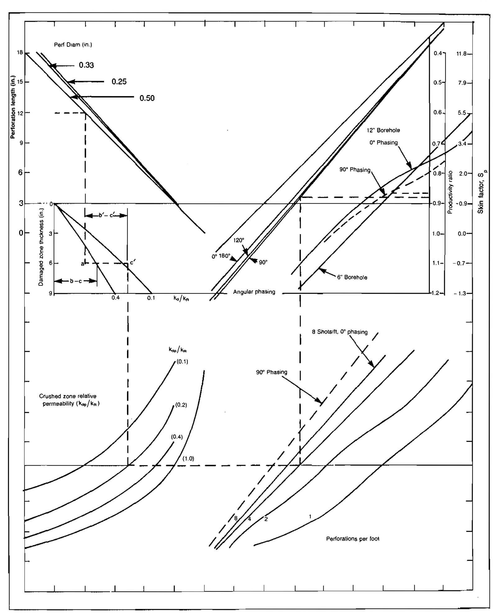
McLeod derived an equation for calculating the effect of flow through the compacted zone as:

S_{d P} = (\frac{h}{L_{P} N}) (\frac{k_{R}}{k_{d P}} - \frac{k_{R}}{k_{d}}) \ln (r_{d P} / r_{P}), E q . 83

where:

h = total formation thickness;
L_P = perforation length;
N = total number of perforations;
k_R = unaltered reservoir permeability;
k_d = altered reservoir permeability;
k_dP = compacted zone permeability;
r_P = perforation radius, and;
r_dP = compacted zone radius.

Picture 31, from Reference 16 shows a schematic of a perforated completion and the relationship among the various parameters in Equation 83.

The largest part of the pressure drop through a perforation is caused by turbulent or non-Darcy flow through the compacted zone. The equation for calculating this effect is:

B_{P} = \frac{3, 161 \cdot 10^{- 12} β_{d P} γ_{g} \bar{Z} T}{r_{P} {L_{P}}^{2} N^{2}} . E q . 84

The value of the velocity coefficient must be calculated using the compacted zone permeability. The equation is:

β_{d P} = \frac{2, 33 \cdot 10^{10}}{{k_{d P}}^{1, 2}} . E q . 85

There are several variables in the equations for perforated completions that are hard to determine. These include the altered zone permeability, the compacted zone permeability, the compacted zone radius, the perforation length, and the altered zone radius. Some of these parameters can be estimated from API-RP-43 test data published by the perforating companies. The following guidelines have been recommended by McLeod:

For wells perforated in mud

\frac{k_{d P}}{k_{R}} = \frac{k_{c}}{k} E q . 86

For wells perforated in brine

\frac{k_{d P}}{k_{d}} = \frac{k_{c}}{k} E q . 87

where k_c/k values are obtained from the API test data. Guidelines for estimating k_c/k when no tests are available were also presented by McLeod in Table 4.

Table 4. Perforating Parameter Guidelines
Fluid in Hole	Pressure Conditions	k_c/k
High solids mud	overbalance	0,01-0,03
Low solids mud	overbalance	0,02-0,04
Unfiltered brine	overbalance	0,04-0,06
Filtered brine	overbalance	0,08-0,16
Filtered brine	underbalance	0,15-0,25
Clean fluid	underbalance	0,30-0,50
Ideal fluid	underbalance	1,00

McLeod also suggests that the compacted zone thickness is usually about 0,5 in. That is, r_dP = r_P+0,5 if r_P is in inches. If no information is available regarding the altered zone radius, a value of r_d = r_w+1 may be used, where r_w is given in ft.

Perforated, Gravel-Packed Completions

The equation for a gravel-packed completion is:

{\bar{p}}_{R}^{2} - {p_{w f}}^{2} = (A_{R} + A_{P} + A_{G}) q_{s c} + (B_{R} + B_{P} + B_{G}) {q_{s c}}^{2} . E q . 88

For most gravel-packed wells the formation will have a high permeability because of the unconsolidated nature of the sand. This will also result in minimum damage from the compacted zone around the perforations. However, the effect of the linear flow through the perforation tunnel that is filled with pack sand can cause a significant non-Darcy flow pressure drop. The equations for A_G and B_G are:

A_{G} = \frac{2 844 \bar{Z} T {\bar{μ}}_{g} L}{k_{G} N {r_{p}}^{2}}, E q . 89

B_{G} = \frac{1, 263 \cdot 10^{- 11} β_{G} γ_{g} \bar{Z} T L}{N^{2} {r_{P}}^{4}}, E q . 90

where:

k_G = gravel permeability, md;
L = perforation tunnel length, ft, and:
$β_{G} = \frac{1, 47 \cdot 10^{7}}{{k_{G}}^{0, 55}} . E q . 91$

The following data, from Gurley, ‘0 may be used to estimate the gravel permeability based on its size.

Sieve Size	kg, md
10-20	5,00·10⁵
16-30	2,50·10⁵
20-40	1,20·10⁵
40-60	4,00·10⁴

A schematic of a gravel packed completion is illustrated in Picture 32.

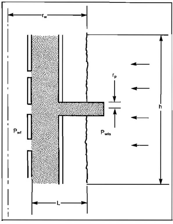
Scheme of gravel-packed completion — Pic. 32 Gravel-packed completion

As illustrated in Picture 32, the tunnel length is defined as the radius of the hole minus the outside radius of the screen. In some cases it is defined as the hole radius minus the inside radius of the casing.

In analyzing gravel-packed completions it is some times convenient to break down the total pressure drawdown into two separate components. That is, the pressure drop in the reservoir and the pressure drop in the gravel pack. This can be expressed as:

{\bar{p}}_{R} - p_{w f} = {\bar{p}}_{R} - p_{w f s} + (p_{w f s} - p_{w f}), E q . 92

where p_wfs is the pressure existing at the sand face, as illustrated in Picture 3-32. Most operators agree that the pressure drop across the gravel pack, p_wfs-p_wf, shoud be below about 300 psi. The equations for the two pressure drops, ignoring A_P and B_P, may be written as:

{\bar{p}}_{R}^{2} - {p_{w f s}}^{2} = A_{R} q_{s c} + B_{R} {q_{s c}}^{2} E q . 93

{\bar{p}}_{w f s}^{2} - {p_{w f}}^{2} = A_{G} q_{s c} + B_{G} {q_{s c}}^{2} E q . 94

This type of analysis may also be applied to nongravel packed completions.

Tight Gas Well Analysis

Predicting the inflow performance for a very low permeability gas well can be difficult because of the necessity to obtain stabilized well tests. As was discussed previously, both the isochronal and modified isochronal tests require one stabilized production point for analysis. Even though the LIT analysis can be used without a stabilized test, using this method to generate a stabilized IPR assumes that the well will eventually stabilize.

If a gas well is draining a fairly large area from a tight reservoir, the well may produce in the unsteady-state flow regime for most of its life. As an example, the stabilization time for a well draining a square or circular area can be estimated from.

t_{s} = \frac{380 ϕ {\bar{μ}}_{g} \bar{C} A}{k} . E q . 33

Consider a well having the following characteristics:

ϕ = 10 %;
A = 640 acres;
${\bar{μ}}_{g}$
= 0,011 cp;
k = 0,05 md;
$\bar{C}$
= 2,5·10^-4psi^-1.

The stabilization time is approximately:

t_{s} = \frac{380 (0, 1) (0, 011) (2, 5 \cdot 10^{- 4}) (640) (43 650)}{0, 05}

t_s = 58,266 hours = 6,65 years

This is of course an extreme case, and a well with permeability this low would require stimulation by a massive hydraulic fracture to be commercial.

A procedure for predicting the inflow performance of a fractured gas well as a function of time was presented by Agarwal, et al., in 1979. The method uses the constant well pressure solution to the diffusivity equation and utilizes computer generated, dimensionless type curves to evaluate the fracture parameters.

A procedure is described to analyze a drawdown test in which the wellbore flowing pressure is held constant and the decline of flow rate with time is measured. The following dimensionless variables are used in analyzing a well with a hydraulic fracture of length X_e = 2X_f. A schematic of the system geometry is shown in Picture 33.

System geometry — Pic. 33 Schematic view of a fractured well

The dimensionless time based on fracture half-length is:

t_{D X} = \frac{0, 000264 k t}{ϕ {(μ C)}_{i} X_{f}^{2}} . E q . 95

The dimensionless flow rate is expressed as:

\frac{1}{q_{D}} = \frac{k h (p_{i}^{2} - {p_{w f}}^{2})}{1 422 q_{s c} \bar{μ} \bar{Z} T}, E q . 96

k = permeability, md;
t = flowing time, hours;
ϕ = porosity;
(μC)_i = viscosity-compressibility product evaluated at p_i, T;
μ = viscosity, cp;
C = total compressibility, psi^-1;
X_f = fracture half-length, ft;
h = formation thickness, ft;
p_i = initial reservoir pressure, psia;
p_wf = flowing wellbore pressure, psia;
q_sc = gas flow rate, Mscfd;
T = reservoir temperature, °R, and;
Z = gas compressibility factor evaluated at
T,
$\bar{p} = (p_{i} + p_{w f}) / 2 .$

A dimensionless fracture flow capacity was defined as:

F_{C D} = \frac{k_{f} w}{k X_{f}} E q . 97

where:

k_f = fracture permeability, md;
k = formation permeability, md;
w = fracture width, ft, and;
X_f = fracture half-length, ft.

Agarwal, et al., presented dimensionless of 1/q_D versus t_DX with F_CD as a parameter. An example curve is shown in Picture 34. Larger versions of this curve are available from the Society of Petroleum Engineers.

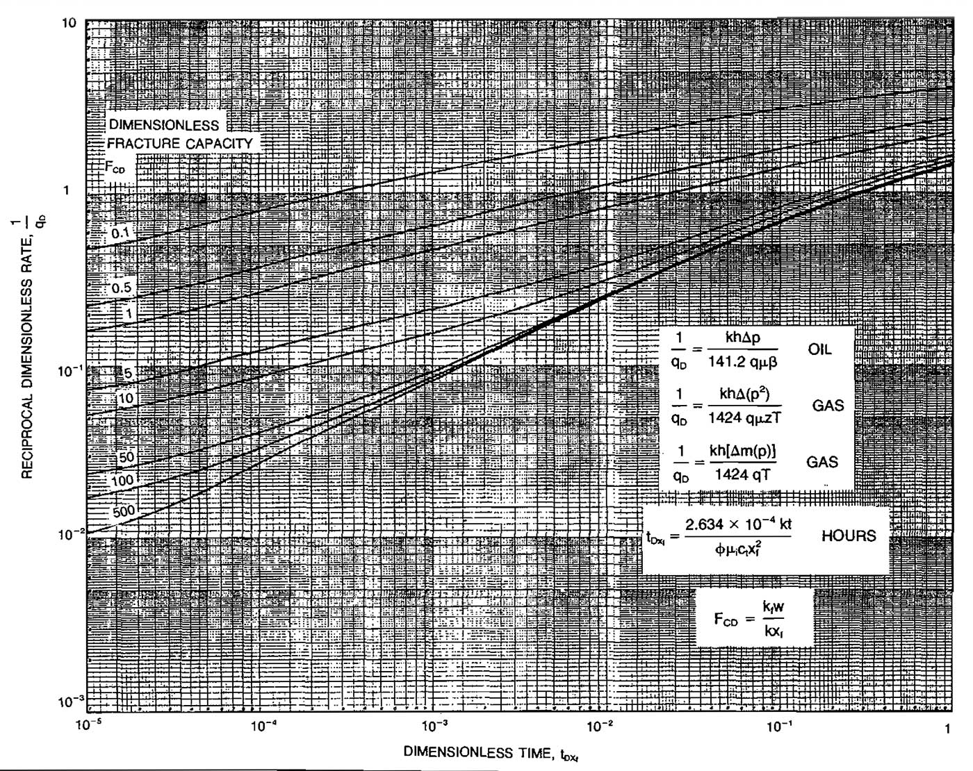
Curve: constant pressure — Pic. 34 Constant-pressure log-log type curves for finite flow-capacity vertical fractures

The following procedure may be used to calculate the production rate versus time and flowing wellbore pressure. A drawdown test is used to evaluate X_f, k and F_CD.

Plot 1/q_sc versus flowing time t on a log-log scale having the same scale as the type curve, Picture 34. It is convenient to use tracing paper to make this plot.
Shift the tracing plot in both the horizontal and vertical directions until a match is obtained between the measured data and one of the curves on the type curve. This determines the correct value of F_CD.
Select a match point at any convenient point on the graph. This establishes a correspondence between t and 1/q_sc and 1/q_D.
Using the known values of t and q_D, calculate k and X_f:
$k = \frac{1 422 q_{s c} \bar{μ} \bar{Z} T}{q_{D} h (p_{i}^{2} - {p_{w f}}^{2})}$
$X_{f} = {[\frac{0, 000264 k t}{ϕ {(μ C)}_{i} t_{D X}}]}^{0, 5}$
The actual fracture flow capacity can then be calculated from:
k_fw = F_CD(kX_f).
To predict future performance:
Select a value for real time t and calculate t_DX using the values of k and X_f obtained in Step 4.
From Picture 34 determine the value of q_D for this t_DX using the correct F_CD curve. F_CD was determined in Step 2.
Calculate the actual flow rate corresponding to this time from:
$q_{s c} = \frac{q_{D} k h (p_{i}^{2} - {p_{w f}}^{2})}{1 422 \bar{μ} \bar{Z} T} .$
Repeat Steps 6 through 8 for various values of time t and P_wf to obtain inflow performance curves applicable at various times. The data may be plotted as shown in Picture 35 if the effect of changing p_wf values is to be considered. To observe the decline in flow rate with time at a constant bottom-hole flowing pressure, a plot such as shown in Picture 36 may be constructed.

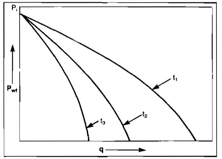
Data plotted — Pic. 35 Inflow performance for various times

The accuracy of the previously described method can be increased somewhat if formation permeability k is known from a pre-frac Horner type analysis. In this case, q_D can be calculated for each real flow rate q_sc, and a plot of 1/q_D versus t can be constructed and used to find a match for the proper F_CD value. The match would then be obtained by shifting the real data curve in the horizontal direction only.

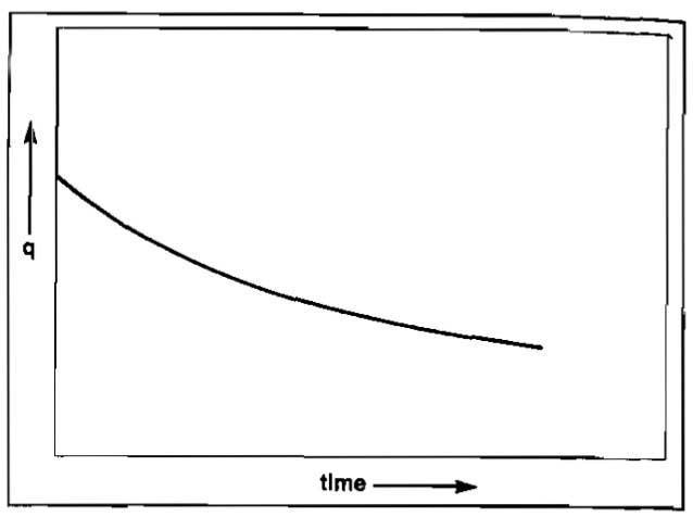
Decline in flow rate — Pic. 36 Producing rate for constant pwf

The procedure outlined here is only one of many methods that may be used for analyzing fractured gas wells. A discussion of all of the methods is beyond the scope of this book.

Guidelines for Gas Well Testing

The accuracy of the results calculated using the previously presented procedures depends on the accuracy of the data used. Obtaining accurate field data can be accomplished only if the field personnel follow established procedures for data collection.

Sweet Dry Gas

The simplest configuration of wellhead testing facilities is required for a well producing a sweet dry gas. The testing equipment essentially consists of a flow rate measurement device, a shut-in and flowing pressure measurement device, a thermometer, gas sampling equipment, and the necessary fittings for connecting the equipment to the wellhead.

When the produced gas is being vented to the atmosphere, a commonly used flow rate measurement device is a critical flow prover that is attached to the top of the wellhead. Unless there are regulations to the contrary, the gas vented from the flow prover is not burned. A horizontal positioning of the flow prover should be avoided since high flow rates will set up a considerable torque that may cause the prover fittings or the wellhead to unwind.

If the well being tested is to be produced into a gas gathering system, the flow rate measurement is usually made with an orifice meter using a permanent or removable meter run.

In some instances, the production well that is to be tested does not have a permanently installed flow measurement device. To avoid interruption of flow or the disruption of stabilized flow in a well that has been producing for some time, a simple procedure illustrated by Picture 37 may be employed.

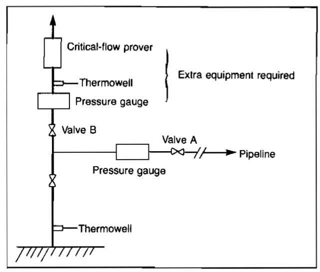
Flow rates of production — Pic. 37 Schematic flow diagram for measuring flow rates of production wells not equipped with flow-rate measurement equipment.

As shown in this picture, if valve A is closed gradually, while valve B is being opened, maintaining a constant pressure in the flow string, the flow rate being measured by the flow prover will be the same as the production rate.

The desirability of constant flow rates during tests is very important. Picture 38 illustrates the wellhead rigging that may provide constant flow rates.

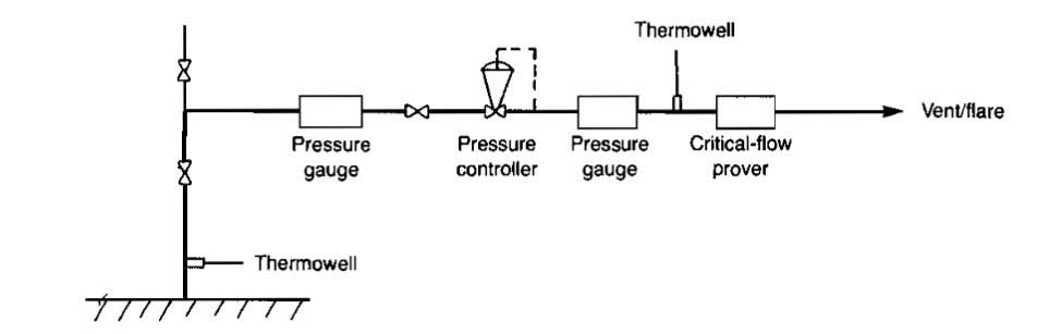
Flow downstream from the flow prover is usually vented to the atmosphere. If, however, the produced gas must be flared, care must be taken to ensure that critical flow conditions are maintained in the flow prover.

The theory and application of the metering devices are discussed in Determination of Volumetric Flow Rates of Gas using Orifice Metering System and other Techniques“Most Common Methods to Measure Gas Flow Rates”.

Sweet Wet Gas

The term “wet” is used to describe a natural gas containing heavier hydrocarbons that appear as a condensate in the produced gas. In some instances, water may also be produced, but it is not included in the definition of a wet gas.

The presence of condensate in produced gas creates requirements for more complex testing facilities than those required for sweet, dry gas wells. A typical facility includes flow rate measurement devices, pressure measurement devices, thermometers, gas and condensate sampling equipment, line heaters, and separation facilities. Several stages of separation and a combination of measurements may be required for highly productive wells, but the most commonly used configurations involve either a single separator or two separators in series. These are illustrated by Pictures 39 and 40, which are intended only as a guide in the selection of test equipment and do not represent the complete wellhead and separation facilities.

Surface well testing — Pic. 39 Schematic flow diagram of surface well testing facilities for wet gas (two separators)

The requirement for line heaters is necessitated by the possibility of hydrate formation within the flow lines and testing equipment.

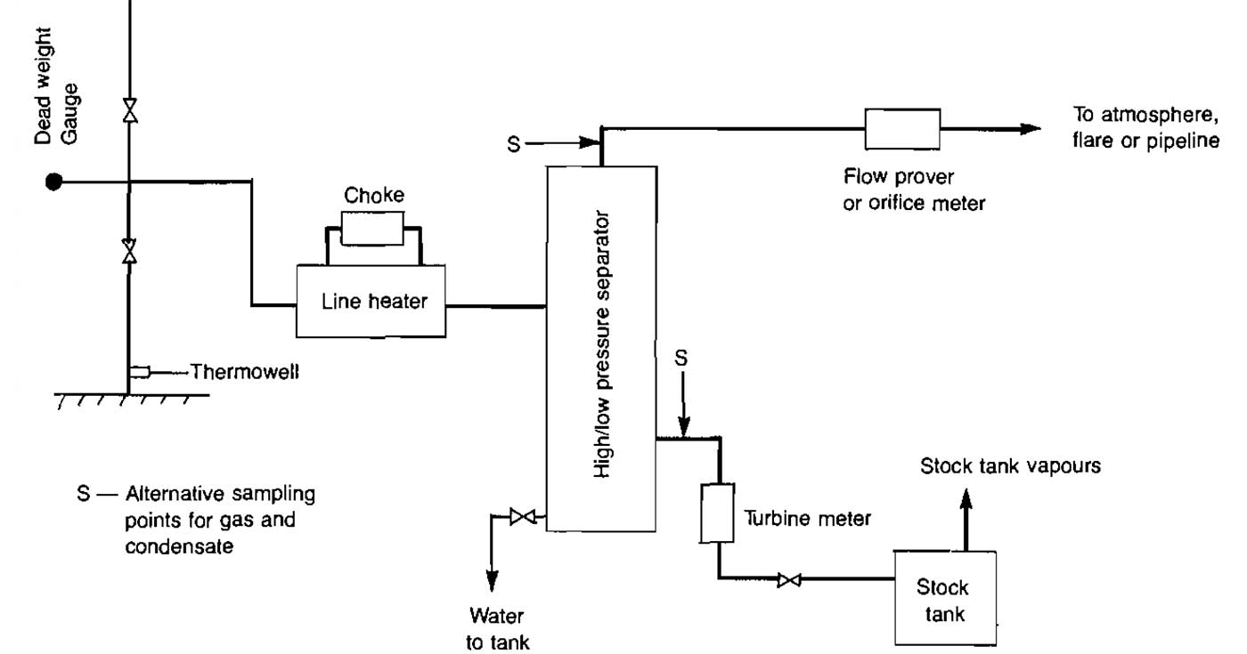
Testing for wet gas — Pic. 40 Schematic flow diagram of surface well testing facilities for wet gas (single separator).

Rather than using a line heater, glycolor alcohol may be injected into the gas stream to prevent the formation of hydrates.

Sour Gas

For testing sour gas wells, more elaborate facilities are required. In addition to the standard equipment, depending on whether the gas is dry or wet, a gas meter and a flow line to an appropriate flare stack are required. In addition, liquid seals may also be necessary to protect the gas meter and pressure measuring device from H₂S gas.

Flow Measuring

The accurate measurement of gas and liquid production rates is essential to the proper conduct and analysis of well tests. Correct sampling procedures are also necessary in order to obtain representative samples of the produced fluids and an accurate estimate of the constituents of the reservoir gas.

All flow measurement devices should be installed in accordance with recommended specifications since biased measurement errors can cause anomalous test results. Some of the more common biased errors are caused by insufficient pipe upstream and downstream of the meter, insufficient liquid retention time in the separators, inadequate liquid dumping cycles, incorrect meter coefficients or calibration factors, meter vibration, and other metering problems.

The most commonly used gas flow measurement devices are orifice meters and critical flow provers. Turbine and displacement meters are not as commonly used, but it is expected that with the advent of portable units their utility will increase.

When the condensate flow rate is being measured, turbine or positive displacement meters are usually used. The meter should be installed with sufficient straight pipe and should be located upstream of a snap-acting valve. This valve should be regulated so that there is sufficient retention time to ensure equilibrium of the gas and liquid in the separator.

In many instances, condensate is gaged in a stock tank. This method should be used only in instances where the input to the stock tank is from a low-pressure separator or when the flashed vapors are being collected. In the former case, care should be taken to ensure that the amount of flashed vapors is small enough to be neglected in recombination calculations.

Water flow rates may be measured with turbine or displacement meters, or gaged in a storage tank. If meters are being used, a snap-acting water dump valve should be used to ensure that there is sufficient flow to activate the meter. Since water, if present in gas, often presents a problem in the operation of gas wells and gas gathering systems, it is important to monitor any water production during a test. A knowledge of water production during tests is also important to the analysis and application of test results.

Pressure Measuring

The accurate measurement of static pressures and the pressures corresponding to flow rates measured during the flow periods of various tests is of great importance in gas well testing. Since interpretation of deliverability, drawdown and build-up test results must be based on the theory of flow in the reservoir, it follows that the important pressure in interpreting the tests is the reservoir sandface pressure (in the wellbore). Ideally, this pressure is measured directly through use of an accurate, carefully calibrated bottom-hole pressure gage. There are many types of such gages available today, all of which, when used properly, are quite adequate for accurate measurement of sandface pressures.

In some instances, due to mechanical difficulties, sour gases, or other reasons, it is not practical to use a bottom-hole gage. In such situations, wellhead pressures are measured and subsequently converted to reservoir sandface pressures by the methods described in Performance of the Network of Pipes in Gas Industry“Performance of Piping System in the Modern Gas Industry”. The highest possible accuracy in wellhead pressure measurement is important, and for best results these pressures should be taken with a dead-weight gage. This is a device that balances the force created by the well pressure with calibrated weights.

Test Design

If a deliverability test is to be conducted on a well, the test designer must make a decision regarding the range of production or flow rates and also the duration of each flow rate. A decision must also be made as to what type of test is better, flow-after-flow or isochronal. If stabilization time is short a conventional flow-after-flow test may be selected, but if the well is producing from a low permeability reservoir or draining a large area, an isochronal or modified isochronal may be more feasible. If estimates of permeability and drainage area can be made, Equation 33 can be used for estimating stabilization time. Equation 33 can also be solved for radius and used to estimate how far a pressure disturbance created at the well will have traveled at a particular time.

A flow-after-flow test requires at least two tests in which the rates are held constant until the well is stabilized. The best indication of stabilization is a constant flowing bottomhole pressure, but unless a surface readout of this pressure is available, the tester must rely on surface indications of stabilized conditions. Some surface indications of stabilization are constant wellhead pressure and constant gas and liquid production rates, although these do not necessarily mean that the bottomhole pressure is remaining constant. If there is considerable doubt as to the stabilization time, an isochronal test should be selected. It should also be kept in mind that any change in pressure or rate during the test creates another pressure disturbance and will require restabilization.

An isochronal test requires at least two transient tests for determining turbulence characteristics and one stabilized test for calculating the laminar flow behavior. Even though the well need not flow past stabilization time during the transient tests, the duration of these tests must be sufficiently long to insure that the measured pressures are not affected by wellbore storage effects and that the pressure disturbance has traveled past any formation damage or stimulation zones. The duration of each transient test should be at least four times longer than the larger of either the wellbore storage time or the time required for the pressure disturbance to have moved 100 feet from the well.

Equation 33 can be used to calculate the time when r = 100 ft, and the following equation can be used to estimate wellbore storage time.

t_{w s} = \frac{36 000 μ V_{w} C_{w}}{k h}

where:

t_ws = wellbore storage time, hrs.;
μ = gas viscosity at average wellbore conditions, cp;
V_w = wellbore volume, ft³;
C_w = gas isothermal compressibility at average wellbore conditions, psi^-1;
k = formation permeability, md, and;
h = formation thickness, ft.

The magnitude of the flow rates selected for the tests must be at least large enough to continuously remove any liquids produced along with the gas. This minimum rate can be estimated with equations presented in the next article. It should also be high enough to result in a wellhead temperature high enough to prevent hydrate formation. When these considerations do not apply, the minimum and maximum flow rates should be selected such that the drawdown in wellhead pressures are approximately 5 percent and 25 percent of the static wellhead pressure. If an estimate of the AOF is available the rates may be selected as about 10 percent and 75 percent respectively, of the AOF. Estimates of the AOF might be obtained from drillstem test data, well log data, or offset well performance. The rate for the stabilized test is often selected to be approximately equal to the anticipated production rate of the well. Consideration of problems such as water coning and unconsolidated formations must be taken in selecting the maximum rate.

Problems in Gas-Well Testing

There are several problems unique in testing gas wells that can result in erroneous results. These problems are discussed from the standpoint of the types of errors that can result in the test data obtained.

Liquid Loading. The problem of liquid loading usually occurs when testing low productivity gas wells with high liquid-gas ratios. Wide variations of surface pressures may indicate liquid loading.

Hydrate Formation. The problem of hydrate formation occurs normally in high pressure gas wells. However, if adequate production equipment is available, this problem can be eliminated by maintaining the wellstream temperature above the hydrate formation temperature. Conditions promoting hydrate formation are discussed in Gas Field Operation Problems and Methods to Deal With ThemGas Production Problems and Methods to Detect Them.

Wet Gas Streams. Sometimes it is necessary to meter a gas stream at the wellhead. Such streams will often deposit liquid in the flow line downstream of the point where the orifice was installed. If the gas gravity is measured on a gas sample obtained at such a downstream point, its value will not represent the gravity of the gas that flowed through the orifice. In this instance, the measured gas gravity must be adjusted to give the gravity of the full stream. This can be accomplished by use of Best and Most Widely Methods to Perform Necessary Calculations with a Gas“Equation”.

Irregular Flow. One of the most frequent difficulties encountered in making accurate gas flow-rate measurements is the rapidly changing flow rates that accompany “slug flow”, freeze-ups, and paraffin deposition in the wellhead choke. Because this problem is frequent and is a source of major error, it deserves special attention.

Adjusting the dampening screw on the differential meter will narrow the span of the differential variations. This should enable the operator to get a better differential reading. The differential pen should not be dampened to a point of no response.

It is a common experience that mercury meters, even though the wells flow steadily, exhibit substantiai but relatively slow variations in differential reading during a 24 hour period because of atmospheric temperature changes. Temperature data may be obtained with a temperature recorder or periodically measured with a thermometer at the meter run. The variation in the flowing temperature factor is approximately 1 percent per 10 °F of variation in temperature.

Sour (H₂S) Gas. Extreme caution should be exercised in handling gases and liquids containing hydrogen sulfide (H₂S). This hazardous substance is highly toxic and under certain concentration can cause illness and death. Special precautions should be taken when testing wells where hydrogen sulfide is present to be assured that exposure will not exceed the safe maximum allowable concentration for the work period required. Selfcontained breathing apparatus should be worn when hydrogen sulfide concentrations are present that might be injurious to health. Safety considerations are discussed in Gas Field Operation Problems and Methods to Deal With Them“Gas Production Problems and Methods to Detect Them”.

Reporting Data

As discussed previously, well test data are used for various purposes. Routine tests for production records may require only a minimum amount of data such as periodic fluid-rate measurements. On the other hand, special tests for equipment evaluation, well evaluation, reservoir evaluation, and state regulatory body requirements require additional data. As a result, a large amount of data may be required. The amount and type of data will vary from state to state in the case of state regulatory body requirements, and will depend on test objectives if needed for evaluation purposes. Therefore, rather than attempt to list data for a particular purpose, a complete list of well test data is given.

Fluid Measurements: gas rate for all streams, Mscf per day or MMscf per day; condensate rate, stock tank barrels per day; water rate, barrels per day; condensate gravity, API (at 60 °F).
Pressure Measurements, psig: flowing wellhead pressure; shut-in wellhead pressure; flowing bottom-hole pressure (sometimes calculated); shut-in bottom-hole pressure (sometimes calculated); atmospheric pressure.
Temperature Measurements, of: bottom-hole temperature; wellhead temperature; stock-tank liquid temperature; atmospheric temperature.
Choke Size, Inches.
Separation conditions, psig and of: number of separators; separator pressures and temperatures; stabilizer pressure and inlet and outlet temperatures.
Time Data-Minutes, Hours, Days: duration of flowing test; length of time on test choke size before test period; shut-in time for pressure measurement.

Footnotes