Types and Design of the Natural Gas Compressors

There are many cases in gas production operations in which the pressure of a gas must be raised to a higher value. As the pressure in a gas reservoir depletes, it will eventually reach a point where it will no longer overcome all the pressure losses in the system and the pressure of the line into which the gas is being delivered.

СодержаниеСвернуть

Types of Compressors
Positive Displacement Compressors
Dynamic Compressors
Ejector Compressors
Compressor Design
Design Methods
Reciprocating Compressors
Power Requirement
Multistaging
Effect of Clearance
Effect of Specific Heat Ratio
Centrifugal Compressors

It is then necessary to add a compressor to the system to supplement the reservoir energy. In this type of application, the suction or intake pressure, and possibly the volume compressed, will change with time even though the discharge pressure may remain constant. Compressors have been used to lower the wellhead pressure below atmospheric, that is, to pull a vacuum on the well in order to obtain maximum rates.

Compressors are also used to overcome the losses incurred in the long distance transportation of natural gas through transmission lines. This may require large capacity machines operating at essentially constant conditions.

The reinjection of gas for pressure maintenance or cycling requires compression of produced gas to a high pressure to move sufficient volumes into the reservoir. Injection of gas into storage fields also requires a compressor capable of operating under a wide range of conditions.

The engineer is concerned with essentially two types of compressor design problems:

determination of the power required to compress a certain volume of gas from some given intake pressure to a given discharge pressure and;
estimation of the capacity of an existing compressor under required pressure increase conditions. It is also frequently necessary to calculate the temperature increase occurring in the gas as it is compressed.

Types of Compressors

The principal types of compressors are positive-displacement, or intermittent flow, units and continuous flow units. Positive-displacement units are those in which successive volumes of gas are confined within a closed space and elevated to a higher pressure. Continuous flow units are those in which a rapidly rotating element accelerates the gas as it passes through the element, converting the velocity head into pressure, partially in the rotating element and partially in stationary diffusers or blades. The principal compressor types are defined below (see Pic. 1).

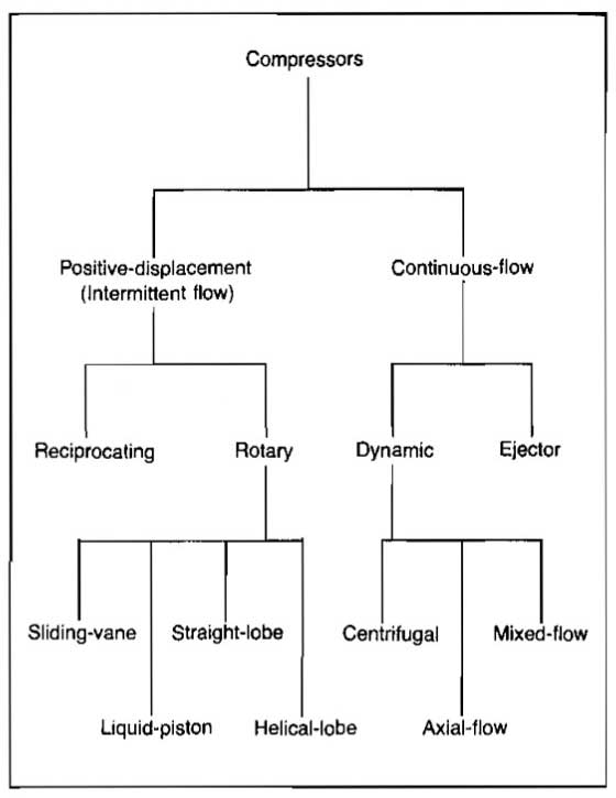
Principal compressor types — Pic. 1 Chart of principal compressor types

Reciprocating compressors are positive-displacement machines in which the compressing and displacing element is a piston having a reciprocating motion within a cylinder.
Rotary positive-displacement compressors are machines in which compression and displacement are effected by the positive action of rotating elements.
Sliding-vane compressors are rotary positive-displacement machines in which axial vanes slide radially in a rotor eccentrically mounted in a cylindrical casing. Gas trapped between vanes is compressed and displaced.
Liquid-piston compressors are rotary positive-displacement machines in which water or other liquid is used as the piston to compress and displace the gas handled.
Two-impeller straight-lobe compressors are rotary positive-displacement machines in which two straight mating lobed impellers trap gas and carry it from intake to discharge. There is no internal compression.
Helical- or spiral-lobe compressors are rotary positive-displacement machines in which two intermeshing rotors, each with a helical form, compress and displace the gas.
Centrifugal compressors are dynamic machines in which one or more rotating impellers, usually shrouded on: the sides, accelerate the gas. Main gas flow is radial.
Axial compressors are dynamic machines in which gas acceleration is obtained by the action of the bladed rotor shrouded on the blade ends. Main gas flow is axial.
Mixed-flow compressors are dynamic machines with an impeller form combining some characteristics of both the centrifugal and axial types.
Ejectors are devices that use a high velocity gas or steam jet to entrain the inflowing gas, then convert the velocity of the mixture to pressure in a diffuser.

Every compressor is made up of one or more basic elements. A single element, or a group of elements in parallel, comprises a single-stage compressor. Many compression problems involve conditions beyond the practical capability of a single compression stage.

Too great a compression ratio (absolute discharge pressure divided by absolute intake pressure) may cause excessive discharge temperature or other design problems. It therefore may become necessary to combine elements or groups of elements in series to form a multistage unit, in which there will be two or more steps of compression. The gas is frequently cooled between stages to reduce the temperature and volume entering the following stage.

Note that each stage is an individual basic compressor within itself. It is sized to operate in series with one or more additional basic compressors, and even though they may all operate from one power source, each is still a separate compressor. The following simplified discussions show the principles of operation of each principal type of compressor.

Positive Displacement Compressors

The basic reciprocating compression element is a single cylinder compressing on only one side of the piston (single-acting). A unit compressing on both sides of the piston (double-acting) consists of two basic single-acting elements operating in parallel in one casting.

The reciprocating compressor uses automatic spring-loaded valves that open only when the proper differential pressure exists across the valve. Inlet valves open when the pressure in the cylinder is slightly below the intake pressure. Discharge valves open when the pressure in the cylinder is slightly above the discharge pressure.

Picture 2, diagram A, shows the basic element with the cylinder full of low pressure gas. On the theoretical pV diagram, point 1 is the start of compression and both valves are closed.

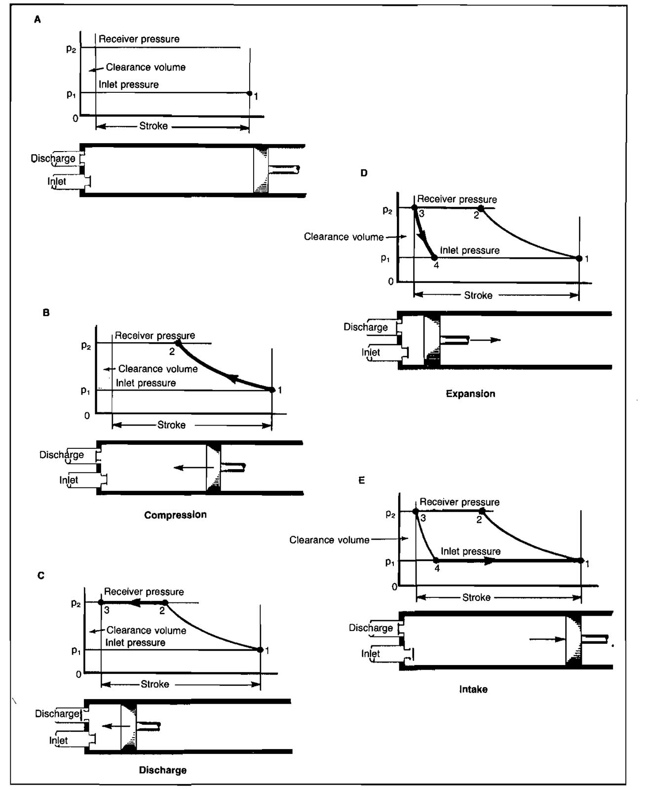
Diagram B shows the compression stroke, the piston having moved to the left, reducing the original volume of gas with an accompanying rise in pressure. Both valves remain closed. The pV diagram shows compression from point 1 to point 2, and that the pressure inside the cylinder has reached that in the receiver.

Diagram C shows the piston completing the delivery stroke. The discharge valve opened just beyond point 2. Compressed gas is flowing out through the discharge valve to the receiver.

After the piston reaches point 3, the discharge valve will close, leaving the clearance space filled with gas at discharge pressure. During the expansion stroke, diagram D, both the inlet and discharge valves remain closed, and gas trapped in the clearance space increases in volume, causing a reduction in pressure. This continues as the piston moves to the right until the cylinder pressure drops below the inlet pressure at point 4. The inlet valve will now open and gas will flow into the cylinder until the end of the reverse stroke at point 1. This is the intake or suction stroke, illustrated by diagram E. At point 1 on the pV diagram, the inlet valve will close, and the cycle will repeat on the next revolution of the crank.

In a simple two-stage reciprocating compressor, the cylinders are proportioned according to the total compression ratio, the second stage being smaller because the gas, having already been partially compressed and cooled, occupies less volume than at the first stage inlet. Looking at the pV diagram (Pic. 3), the conditions before starting compression are points I and 5 for the first and second stages, respectively, after compression, points 2 and 6, and after delivery, 3 and 7.

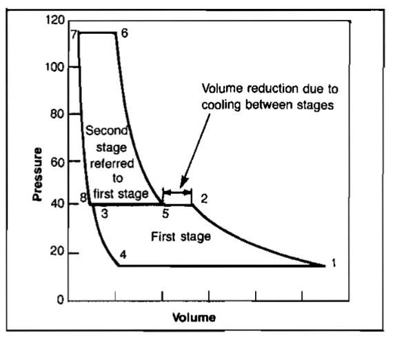
Positive-displacement compressor — Pic. 3 Combined theoretical indicator card for a two-stage, two-element 100 psig positive-displacement compressor

Expansion of gas trapped in the clearance spaces as the pistons reverse brings the pressures and volumes to points 4 and 8, and on the intake stroke the cylinders are again filled at points 1 and 5, and the cycle is set for repetition. Multiple staging of any positive displacement compressor follows this pattern.

The rotary sliding-vane compressor has as its basic element the cylindrical casing with its heads and rotor assembly. When running at design pressure, the theoretical pV diagram is identical to the reciprocator. There is one difference of importance, however. The sliding-vane machine has no valves. The times in the cycle when the inlet and discharge are open are determined by the location of ports over which the vanes pass (Pic. 4).

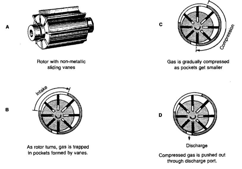
Compression steps — Pic. 4 The steps in compression for a sliding-vane rotary compressor

The pocket volume decreases as the rotor turns and the gas is compressed. Compression continues until the discharge port is uncovered by the leading vane of each pocket. This point must be preset or built-in when the unit is manufactured. Thus, the compressor always compresses the gas to design pressure, regardless of the pressure in the receiver into which it is discharging.

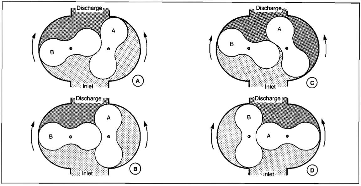
A two-impeller straight-lobe positive-displacement compressor element consists of a casing containing duplicate symmetrical rotors or impellers usually having a figure eight cross section. These intermesh, are kept in phase by external timing gears, and rotate in opposite directions.

There is no compression or reduction of gas volume during the turning of the rotors. The rotors merely move the gas from the inlet to the discharge. Compression is by backflow into the casing from the discharge line at the time the discharge port is uncovered. Displacement of the compressed gas into the discharge system then takes place. There is no contact between the impellers or between impellers and casing. Sealing is by close clearances and lubrication is not required within the gas chamber. One impeller is driven directly while the other is driven through phasing gears. The operation can be visualized from the diagrams of Picture 5. Light shading shows gas at inlet pressure. Dark shading shows gas at discharge pressure.

Inlet and discharge pressure — Pic. 5 The operating cycle of a two-impeller straight-lobe rotary compressor

There are several other types of positive displacement compressors available, as indicated in Picture 1. Most of these are seldom used in the gas industry and are not described.

Dynamic Compressors

Compression in any dynamic compressor depends on the transfer of energy from a rotating set of blades to the gas. The rotor accomplishes this energy transfer by changing the momentum and pressure of the gas. The momentum (related to kinetic energy) then is converted into useful pressure energy by slowing the gas down in a stationary diffuser or another set of blades.

The centrifugal designation is used when the gas flow is radial, and the energy transfer is predominantly due to a change in the centrifugal forces acting on the gas.

The axial designation is used when the gas flow is parallel to the compressor shaft. Energy transfer is caused by the action of a number of rows of blades on a rotor, each row followed by a fixed row fastened to the casing.

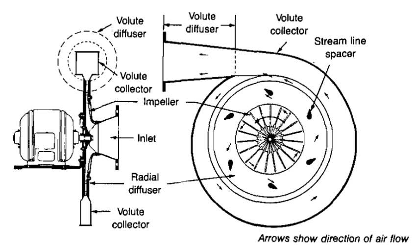
The centrifugal compressor has an impeller with radial or backward slanted vanes usually between two shrouds. The gas is forced through the impeller by the mechanical action of the rapidly rotating impeller vanes. The velocity generated is converted into pressure. Picture 6 illustrates a single-stage centrifugal compressor with radial vanes. This utilizes a radial diffuser and a volute gas collector ending in a volute diffuser.

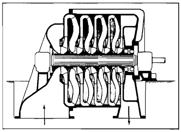
Scheme of single-stage centrifugal compressor — Pic. 6 Typical overhung impeller single-stage centrifugal compressor

Multistage centrifugal compressors utilize two or more impellers arranged for series flow, each with a radial diffuser and return channel separating impellers. The number of impellers per casing is dependent upon many factors, but usually eight to ten is the limit. Picture 7 shows a section of a typical uncooled multistage compressor.

Scheme of uncooled centrifugal compressor — Pic. 7 Cross-section of a typical multistage uncooled centrifugal compressor

An axial-flow dynamic compressor is shown in Picture 8.

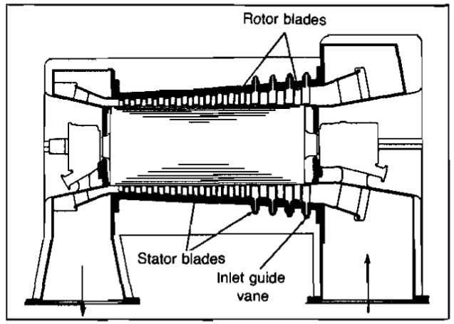
Scheme: dynamic compressor — Pic. 8 Cross-section of a typical axial-flow dynamic compressor

It is essentially a large-capacity high-speed machine with characteristics quite different from the centrifugal. Each stage consists of two rows of blades, one row rotating and the next row stationary. The rotor blades impart velocity and pressure to the gas as the rotor turns, the velocity being converted to pressure in the stationary blades. Frequently about half the pressure rise is generated in the rotor blades and half in the stator. Picture 8 shows a multistage unit. Gas flow is predominantly in an axial direction, there being no appreciable vortex action.

Ejector Compressors

An ejector consists of a relatively high-pressure motive steam or gas nozzle discharging a high-velocity jet across a suction chamber into a venturi-shaped diffuser. The gas, whose pressure is to be increased, is entrained by the jet in the suction chamber. The mixture at this point has high velocity and is at the pressure of the induced gas. Compression takes place as velocity energy us transformed into pressure inside the diffuser.

Ejectors are principally used to compress from pressures below atmospheric to a discharge pressure close to atmospheric. They may, however, involve compression from a near atmospheric intake to some higher level.

A vacuum ejector, using steam as motive fluid and compressing air, is shown in Picture 9. Pressure and velocity changes are indicated for various sections of the device. Temperature changes follow the pressure curve closely.

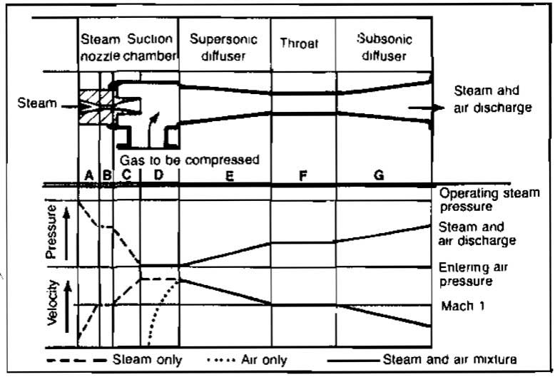
Scheme: vacuum ejector — Pic. 9 A diagram of the pressure and velocity variations within a steam jet ejector handling air

Ejectors have no moving parts. They can handle liquid carry-over without physical damage although they should not be exposed to a steady flow of liquid.

Compressor Design

The principal compressor design problems are the determination of compressor capacity and the determination of power requirements. In making the calculations for these designs, various simplifying assumptions can be made. There are three methods of design:

Analytical expressions;
Mollier diagrams and;
Quick estimates.

The best method in any given situation depends on both the degree of accuracy required and the data available. Detailed design procedures are given for reciprocating and centrifugal compressors only.

Design Methods

Two basic compression cycles or processes are applicable to both positive displacement and dynamic compressors. Although neither of the two basic processes is commercially attainable, they are useful as a basis for calculations and comparisons.

Isothermal compression occurs when the temperature is kept constant as the pressure increases. This requires continuous removal of the heat of compression. The compression process follows the formula.

p_{1} V_{1} = p_{2} V_{2} = Constant . E q . 1

However, it is never commercially possible to remove the heat of compression as rapidly as it is generated.

Adiabatic compression is obtained when there is no heat added to or removed from the gas during compression. The compression process is expressed by Equation 2.

p_{1} V_{1}^{k} = p_{2} V_{2}^{k} . E q . 2

The factor k is the ratio of specific heat at constant pressure to the specific heat at constant volume.

Determination of k for a gas was discussed in Performance of the Network of Pipes in Gas Industry“Performance of Piping System in the Modern Gus Industry”.

Adiabatic compression is likewise never exactly obtained, since with some types of units there may be heat loss during part of the cycle and heat gain during another part. With other types of compressors there may be a definite heat gain. Nevertheless, the adiabatic cycle is rather closely approached with most positive-displacement units and therefore they are usually designed using the adiabatic cycle.

Dynamic units generally are designed based on the polytropic cycle where the pV relationship is:

p_{1} V_{1}^{n} = p_{2} V_{2}^{n} . E q . 3

The exponent n is experimentally determined for a given type of machine and may be lower or higher than the adiabatic exponent k. In positive displacement and internally cooled dynamic compressors n is usually less than k. In uncooled dynamic units it is usually higher than k due to internal gas friction. Although n actually changes during compression, an average or effective value, calculated from experimental information, is used.

Thermodynamically, the isentropic or adiabatic process is reversible, while the polytropic process is irreversible. Also, all compressors operate on a theoretical steady-flow process.

Although the exponent n is seldom required, the quantity (n-1)/n is frequently needed. This can be obtained from the following equation, although it is necessary that the polytropic efficiency (η_p) be known (or approximated) from a prior test. The k value of any gas or gas mixture is either known or can be calculated.

\frac{n - 1}{n} = \frac{k - 1}{k η_{p}}, E q . 4

Either n or (n-1)/n can also be experimentally calculated from test data if inlet and discharge pressures and temperatures are known. The following formula may be used:

\frac{T_{2}}{T_{1}} = {(\frac{p_{2}}{p_{1}})}^{(n - 1) / n} = r^{(n - 1) / n} . E q . 5

This equation may also be used to estimate discharge temperatures when n or (n – 1)/n is known.

It is obvious that k and n can have quite different values. There has been a tendency in the past to use these symbols interchangeably to represent the ratio of specific heats. This is incorrect, and the difference between them should be carefully observed. In the absence of experimental data, an approximation of the polytropic compression efficiency can be obtained from Picture 10.

Picture 11 shows the theoretical zero clearance isothermal and adiabatic cycles on a pV basis for a compression ratio of four. The area ADEF represents the work required when operating on the isothermal basis, and ABEF, the work required when operating on the adiabatic basis. Obviously, the isothermal area is considerably less than the adiabatic and would be the desired cycle for greatest compression economy.

In addition to the isothermal and adiabatic compression curves shown in Picture 11, the dotted lines show typical polytropic curves for a water-cooled reciprocating cylinder (AC) and for a noncooled dynamic unit (AC^′).

All basic compressor elements, regardless of type, have certain limiting operating conditions. When any limitation is involved it becomes necessary to multistage the compression process. Each stage will utilize at least one basic element designed to operate in series with the other elements of the machine.

The limitations vary with the type of compressor, but the most important include:

Discharge temperature – all types;
Pressure rise (or differential) – dynamic units and most positive-displacement types;
Compression ratio-dynamic units;
Effect of clearance-reciprocating units, and;
Desirability of saving power.

A reciprocating compressor usually requires a separate cylinder for each stage, with intercooling of the gas between stages. In a reciprocating unit, all cylinders are commonly combined, into one-unit assembly and driven from a single crankshaft.

It was previously noted that the isothermal cycle is more economical of power. Cooling the gas after partial compression to a temperature equal to original intake temperature obviously will reduce the power required in the second stage.

Dynamic compressors would, in most cases, have several staging elements in the same casing. There would normally be no intercooling between those stages contained in a given casing although the internal diffusers or diaphragms are sometimes water-cooled. The gas can be brought out to external exchangers for intercooling at the end of several stages of compression. Frequently, large units have two casings (separate machines) in series to cover the entire compression range, each machine equipped with several stages and with external intercooling between the machines. They are usually coupled in tandem to one driver. The extent to which intercooling is used depends largely on power cost.

Reciprocating Compressors

As stated earlier, the capacity and power required are the two principal factors that must be determined in designing compressors. Temperature increase and cooling requirements are also frequently required. Several methods for calculating required power are presented in this section. Also, the effect of changing conditions, such as clearance, specific heat ratio, and compressibility are discussed.

Capacity. The amount of gas a given compressor can pump depends on the actual displacement volume of the intake cylinder and the volumetric efficiency. Since all of the gas is not discharged from the cylinder because of the clearance between the piston and the cylinder, the total volume of the cylinder is not available for new gas. The capacity of a compressor is calculated from:

q = \frac{π d^{2} L S E_{v}}{4}, E q . 6

where:

q = flow capacity;
d = piston diameter;
L = stroke length;
S = compressor speed, and;
E_v = volumetric efficiency.

On double-acting compressors the volume occupied by the rod must be accounted for. The volumetric efficiency is calculated from:

E_{v} = 1 - A - C [\frac{Z_{1} r^{1 / k}}{Z_{2}} - 1], E q . 7

where:

A = factor to allow for leakage, friction, etc., usually between 0,03 and 0,06;
C = clearance, which varies from 0,04 to 0,16;
Z₁ = gas compressibility factor at suction conditions;
Z₂ = gas compressibility factor at discharge conditions;
r = compression ratio, p₂/p₁;
p₁ = suction pressure, and;
p₂ = discharge pressure.

Equations 6 and 7 are applicable for any consistent set of units.

Example 1:

A single acting reciprocating compressor having a piston diameter of 4 in. and a stroke length of 6 in. is to compress gas from 100 psig and 100 °F to 400 psig. Calculate the flow capacity in scfd if the compressor runs at a speed of 500 rpm. Other data are:

k = 1,3;
C = 6 %;
A = 5 %.

Solution:

r = p₂/p₁ = 414,7/114,7 = 3,62

T₂ = T₁ r^(k-1)/k = (100+460)(3,62)^.23 = 753 °R

Z₁ = 0,98, Z₂ = 0,95, Z₁/Z₂ = 1,03

E_v = 1-.05-.06 [1,03(3,62)^.77-1] = 0,85

q = π(4/12)²(6/12)(500)(.85)/4 = 18,54 ft³/min

q = 18, 54 \frac{{ft}^{3}}{\min} \cdot \frac{1 440 \min}{day} = 26 704 {ft}^{3} / day

q_{s c} = \frac{q}{B_{g}} B_{g} = \frac{. 0283 Z T}{p} = \frac{. 0283 (. 98) (560)}{114, 7}

B_g = 0,135 ft³/scf

q_{s c} = \frac{26 704}{0, 135} = 1, 97 \cdot 10^{5} scfd

Power Requirement

The power requirement of any compressor is the prime basis for sizing the driver and for selection and design of compressor components. The actual power requirement is related to a theoretical cycle through a compression efficiency that has been determined by tests on prior machines. Compression efficiency is the ratio of the theoretical to the actual gas horsepower, and as used by the industry, does not include mechanical friction losses. These are added later either through the use of a mechanical efficiency or by adding actual mechanical losses previously determined. The mechanical efficiencies of positive-displacement compressors range from 88 to 95 %, depending upon the size and type of unit. Dynamic units also have certain relatively small hydraulic losses that are often disregarded for estimating purposes. Positive-displacement machines are designed based on the adiabatic cycle while dynamic units generally are designed using the polytropic cycle.

In calculating horsepower, the compressibility factor, Z, must be considered since its influence is considerable with many gases, particularly at high pressure. The power required may be determined using analytic equations or Mollier diagrams. Charts for quick estimates are also available. The equations are derived by starting with the general energy equation. Neglecting potential and kinetic energy changes and friction losses, the equation becomes.

w = \int_{p_{1}}^{p_{2}} V d p . E q . 8

To integrate this equation a relationship between V and p must be used. For adiabatic flow, pV^k = constant, and upon integrating, adjusting for gas compressibility and units, the following equation can be obtained:

w = \frac{3, 027 p_{s c} T_{1} k}{T_{s c} (k - 1)} (r^{Z_{1} (k - 1) / k} - 1), E q . 9

where:

w = power required, Hp/MMscfd;
p_sc = pressure at standard conditions, psia;
T_sc = temperature at standard conditions, °R, and;
T₁ = suction temperature, °R.

Example 2:

Calculate the horsepower required to compress 1 MMscfd of a 0,6 gravity gas from 100 psia and 80 °F to 1 600 psia using the adiabatic equation. Assume that a two stage compressor is used, and that the gas is cooled back to 80 °F between stages. Also find the final discharge temperature.

Other data are:

k = 1,28;
p_sc = 14,65;
T_sc = 60 °F.

Solution:

The total compression ratio is 1 600/100 = 16. Therefore, use a value of r = 4 for each stage.

First Stage

p₁ = 100, p₂ = 400, Z₁ = 0,985,

\frac{Z_{1} (k - 1)}{k} = 0, 22

w = \frac{3, 072 (14, 65) (540) (1, 28)}{520 (. 28)} [{(4)}^{0, 22} - 1]

w_{1} = 210, 5 (0, 36) = 75, 8 Hp / MMscfd

The gas temperature after compression from 100 to 400 psia is:

T₂ = T₁ r^(k-1)/k = 540(4)^.22 = 733 °R = 273 °F

The gas is cooled to 80 °F before entering the second stage.

Second Stage

p₁ = 400 psia, p₂ = 1 600 psia, Z₁ = 0,94

\frac{Z_{1} (k - 1)}{k} = 0, 21

w₂ = 210,5(4^.21-1) = 71,6 Hp/MMscfd

T₂ = T_final = 273 °F

The total power required is:

Hp = q(w₁+w₂) = 1 MMscfd (75,8+71,6) Hp/MMscfd

Hp = 147,4

In order to size the prime mover for the compressor a compression efficiency must be estimated. Picture 12 can be used for determining efficiency as a function of the compression ratio. From Picture 12, for r = 4, E = 83 %. Therefore, the actual brake horsepower required is:

b h p = \frac{147, 4}{0, 83} = 177, 6 .

Power requirement and cooling requirements can be determined using plots of enthalpy versus entropy (Mollier diagrams) if a plot is available for the gas that is to be compressed. When cooling the gas, which occurs at constant pressure, the change in enthalpy can be used to determine the amount of heat to be removed. From thermodynamics:

ΔH = Q-w, Eq. 10

where:

ΔH = change in enthalpy;
Q = heat transferred during compression, and;
w = work.

For adiabatic compression, Q = 0 and:

-w = ΔH. Eq. 11

In units of horsepower per million standard cubic feet, Equation 11 becomes:

w = 0,0432 ΔH, Eq. 12

where:

w = power required, Hp/MMscfd, and;
ΔH = enthalpy change, BTU/lb-mole.

When cooling the gas, w = 0 and therefore:

Q = ΔH, Eq. 13

Example 3:

Use the Mollier diagram method to solve Example 2. Also calculate the heat to be removed between stages to cool the gas to 80 °F.

Solution:

Select Picture 13 to represent the gas.

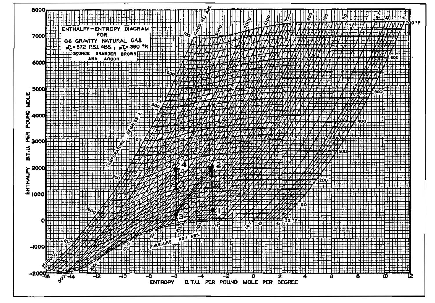
Pic. 13 Enthalpy-entropy diagram for 0,6 gravity natural gas

First Stage

The first stage compresses the gas from 100 psia to 400 psia at constant entropy. Enter Picture 13 at p₁ = 100 and T₁ = 80 °F and read H₁ = 380 BTU/lb-mole. Proceed vertically (ΔS = 0) to p₂ = 400 psia and read H₂ = 1 990, T₂ = 260 °F. Follow the 400 psia line to T₃ = 80 °F and read H₃ = 220. The amount of cooling required is then:

Q = ΔH₂₃ = H₂-H₃ = 1 990-220 = 1 770 BTU/lb-mole,

or:

Q = 1 770 \frac{BTU}{lb - mole} \cdot \frac{lb - mole}{379 scf} = 4, 67 \frac{BTU}{scf}

The power required for stage 1 is:

w = 0,0432 ΔH₁₂ = 0,0432(H₂-H₁)

w = 0,0432(1 990-380) = 70 Hp/MMscfd

Second Stage

From point 3 where:

p = 400,
T = 80 and,
H = 220,

proceed vertically to the final pressure of 1 600 psia and read T₄ = 274 °F, H₄ = 1 920 BTU/lb-mole. The power required for the second stage is then:

w = 0,0432(H₄-H₃) = 0,0432(1 920-220) = 73,4 Hp.

The total horsepower required is then:

Hp_total = q(w₁+w₂) = 1 MMscfd (70+73,4) = 143,4

This compares well with the value of 147,4 Hp obtained using the equations. The Mollier diagram solution is considered to be more accurate and should preferably be used. Mollier diagrams for other gases are included in the appendix.

For making rough estimates of power requirement the following equation can be used:

bhp = 22 r N q_sc F Eq. 14

where:

bhp = brake horsepower;
r = compression ratio per stage;
N = number of stages;
q_sc = flow rate in MMscfd, and;
F = correction for pressure drop between stages, depending on N.

N	F
1	1,00
2	1,08
3	1,10

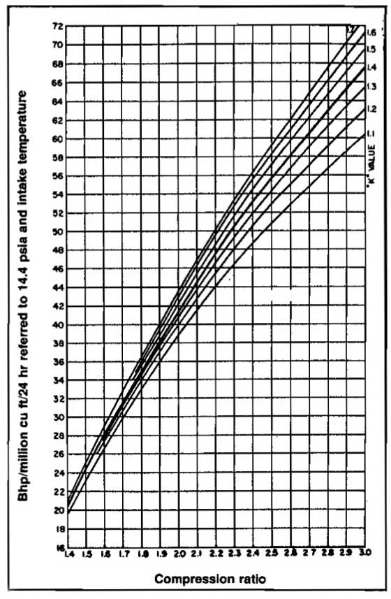
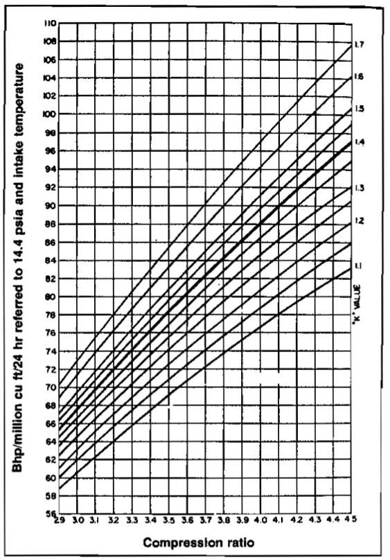
Graphical solutions to Equation 9 have been prepared for specific conditions of compression efficiency, standard conditions, and gas gravity. Examples are shown in Pictures 14 through 16.

Example of compressor power requirements — Pic. 14 Compressor power requirements

Diagram: compressor power requirements — Pic. 15 Compressor power requirements

Power requirements — Pic. 16 Compressor power requirements

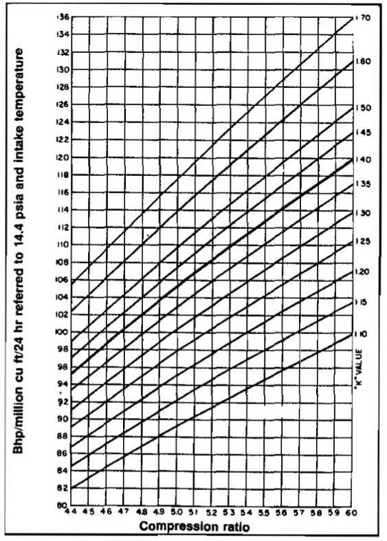
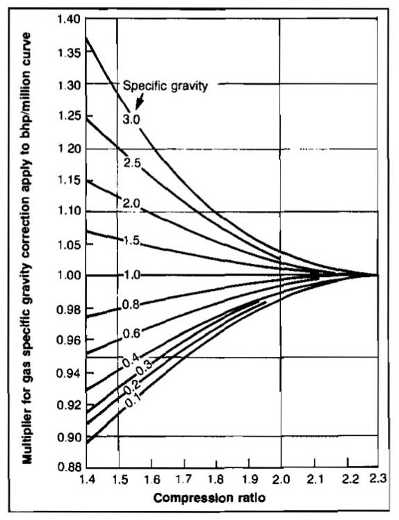
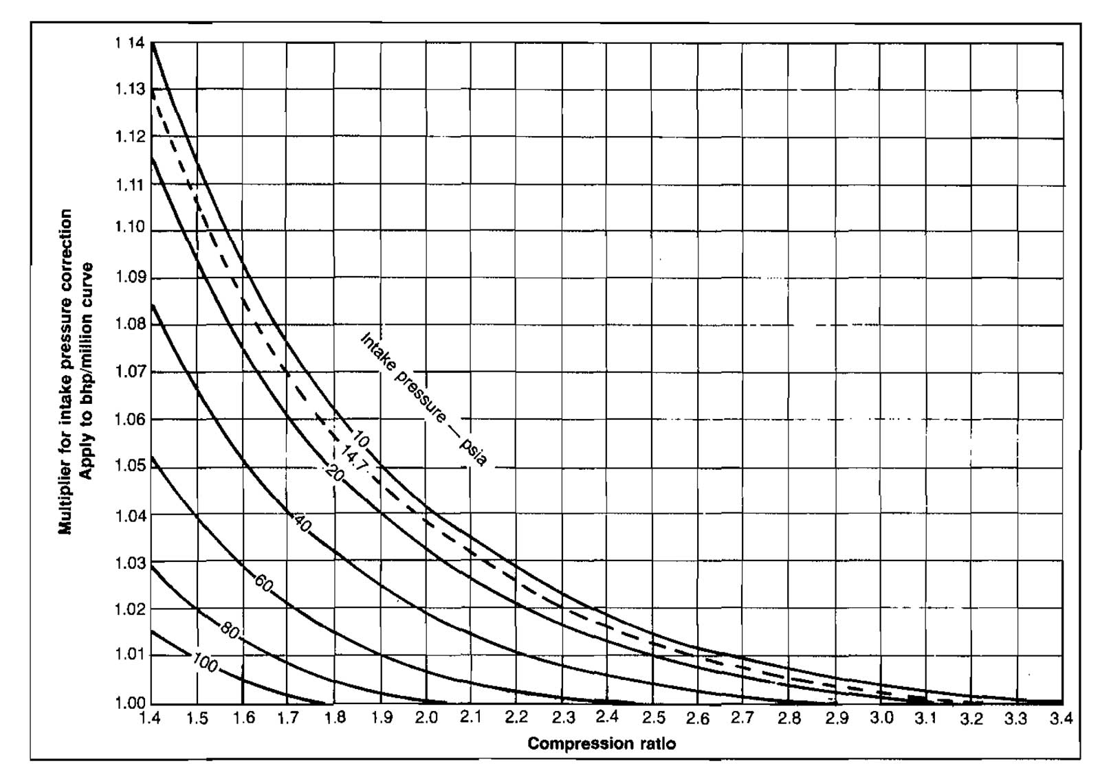
Correction to other gas gravities and for low suction pressure are obtained from Pictures 17 and 18 respectively.

Correction to the gas gravity — Pic. 17 Specific gravity correction

Graph: pressure correction — Pic. 18 Suction pressure correction

Example 4:

Solve Example 2 using both Equations 14 and the graphs presented in Pictures 14 through 16.

q_sc = 1 MMscfd;
p₁ = 100 psia;
p₂ = 1 600 psia;
k = 1,28;
γ_g = 0,6.

Solution:

Using Equation 14, bhp = 22(4)(2)(1)(1,08) = 190 Hp.

Using Picture 15, for r = 4 and k = 1,28, read bhp/MMscfd = 84. For 2 stages this will be 2(84) = 168 Hp. There is no correction for low suction pressure or gas gravity since r is greater than 3, 4, the limit of the correction graphs.

Multistaging

It has been previously stated that there are practical limits to the amount of compression permissible within a single stage or element beyond which two or more steps or stages must be used with intercooling between stages in most cases.

Theoretically minimum power with perfect intercooling and no pressure loss between stages is obtained by making the ratio of compression the same in all stages. The following formula may be used to determine the optimum compression ratio per stage:

r_{s} = \sqrt[s]{r_{t}} = {(r_{t})}^{1 / s} E q . 15

where:

r_s – is the theoretically best compression ratio per stage;
r_t – is the overall compression ratio
$(\frac{p_{f i n a l}}{p_{i n i t i a l}}),$
and;
s – is the number of stages.

Even though this method results in minimum power, the energy required will vary only a fraction of one percent for rather large variations in the actual compression ratios for individual stages. Designers take advantage of this fact for economic and engineering reasons.

Each stage is best designed as a separate compressor, the capacity of each stage being separately calculated from the first stage real intake volume, corrected to the actual pressure and temperature conditions existing at the higher stage cylinder inlet, allowing for pressure drop through cooler and piping. Allowances must also be made for any reduction in the moisture content if there is condensation between stages in an intercooler. The theoretical power per stage can then be calculated and the total horsepower obtained. A compression ratio per stage greater than four is seldom used because of heating and rod loading problems.

Effect of Clearance

Although cylinder clearance reduces the volumetric efficiency of a compressor (Eq. 7), it cannot be completely eliminated. Clearance may be altered for capacity control. Pictures 19 and 20 show the effect of clearance by means of a pV diagram.

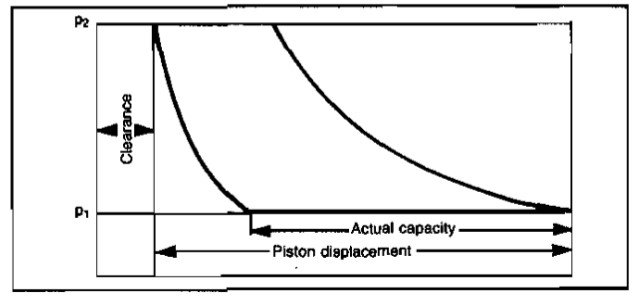
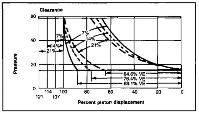
Scheme: cylinder clearance — Pic. 20 Quantitative effect of various cylinder clearances on the volumetric efficiency at constant compression ratio

Picture 21 illustrates how the clearance may be varied to alter volumetric efficiency and therefore capacity.

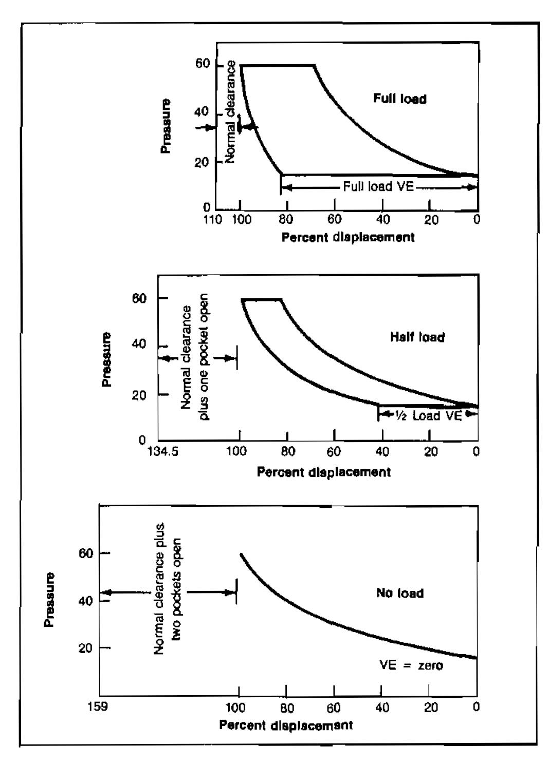
Altering volumetric efficiency and therefore capacity — Pic. 21 Effect of adding clearance for capacity purposes

Actual clearance control is accomplished by adding pockets or bottles to the cylinder, which may be open or closed, or by adjustable clearance valves.

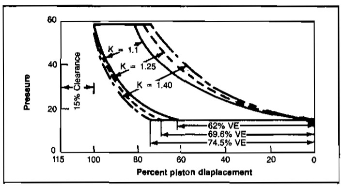
Effect of Specific Heat Ratio

Picture 22 shows the effect of specific heat ratio, k = C_p/C_v, on volumetric efficiency for a fixed compression ratio and clearance. The lower the value of k, the lower the volumetric efficiency.

Centrifugal Compressors

The performance of a centrifugal compressor is usually estimated based on the polytropic process. The same equation (Eq. 9) given for a reciprocating compressor can be used if k is replaced with n, where:

\frac{n - 1}{n} = \frac{k - 1}{k η_{p}} . E q . 4

The concept of polytropic head is frequently used in designing centrifugal machines since the head developed is independent of the fluid being moved. The polytropic head is the work in energy per unit mass of the gas. It can be calculated from:

H_{p} = \frac{R T_{1} n Z}{M (n - 1)} (r^{(n - 1) / n} - 1), E q . 16

where:

H_p = polytropic head;
R = gas constant;
T₁ = gas inlet temperature;
$\bar{Z}$
= average compressibility factor, (Z₁ + Z₂)/2, and;
M = gas molecular weight.

The actual power required then depends on the amount of gas being moved, or the mass flow rate, w. In terms of horsepower:

Hp = \frac{w H_{p}}{33 000 η_{p}}, E q . 17

where:

Hp = power required, horsepower;
w = mass flow rate, lb_m/min;
H_p = polytropic head, ft-lb/lb_m, and;
η_p = polytropic efficiency.

In determining the brake horsepower required, mechanical losses must be added. These will usually vary between 10 and 50 Hp, depending on the machine. The power required can also be obtained using a Mollier diagram, as outlined previously in the discussion of reciprocating compressors.

Example 5:

Using the following data, estimate the horsepower required for a centrifugal compressor to compress 50 MMscfd of a 0,6 gravity gas.

p₁ = 100 psia;
p₂ = 400 psia;
p_sc = 14,65 psia;
Z₁ = 0,988;
T₁ = 80 °F;
k = 1,28;
T_sc = 60 °F;
B_gl = 0,131 ft³/scf.

Solution:

The actual inlet volume is:

q = q_{s c} B_{g} = 50 \cdot 10^{6} \frac{scf}{day} \cdot 0, 131 \frac{{ft}^{3}}{scf} \cdot \frac{day}{1 440 \min}

From Picture 10, η_p = 0, 72:

\frac{n - 1}{n} = \frac{k - 1}{k η_{p}} = \frac{1, 28 - 1}{1, 28 (0, 72)} = 0, 3

T_{2} = T_{1} r^{(n - 1) / n} = 540 {(4)}^{0, 3} = 818 ° R

Z_{2} = 0, 991 \bar{Z} = \frac{0, 988 + 0, 991}{2} = 0, 99

M = 28,96 γ_g = 28,96(.6) = 17,38 lbm/lb-mole

H_{p} = \frac{R T_{1} n \bar{Z}}{M (n - 1)} (r^{(n - 1) / n} - 1)

H_{p} = \frac{1 545 (540) (. 99)}{17, 38 (0, 3)} ({(4)}^{0, 3} - 1) = 81 700 \frac{ft - lb}{lbm}

w = 50 \cdot 10^{8} \frac{scf}{day} \frac{17, 38 lbm}{379 scf} \frac{1 day}{1 440 \min} = 1 592 \frac{lbm}{\min}

H p = \frac{w H_{p}}{33 000 η_{p}} = \frac{1 592 (81 700)}{(33 000) (0, 72)} = 5 474 H p

Estimates of the horsepower, number of stages, and compressor speed can be made by referring to Pictures 23 through 26.

Diagram: basic horsepower — Pic. 23 Basic horsepower

Diagram: value correction — Pic. 24 K value correction

Diagram: basic head — Pic. 25 Basic head

Diagram: compressor speed — Pic. 26 Compressor speed

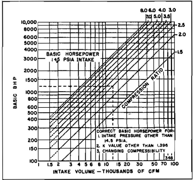
The horsepower required for a centrifugal compressor is obtained from:

H p = (BASIC BHP) \frac{p_{1} \bar{Z}}{14, 5 Z_{1}} (K_{c o r r})

where:

(BASIC BHP) – is obtained from Picture 23;
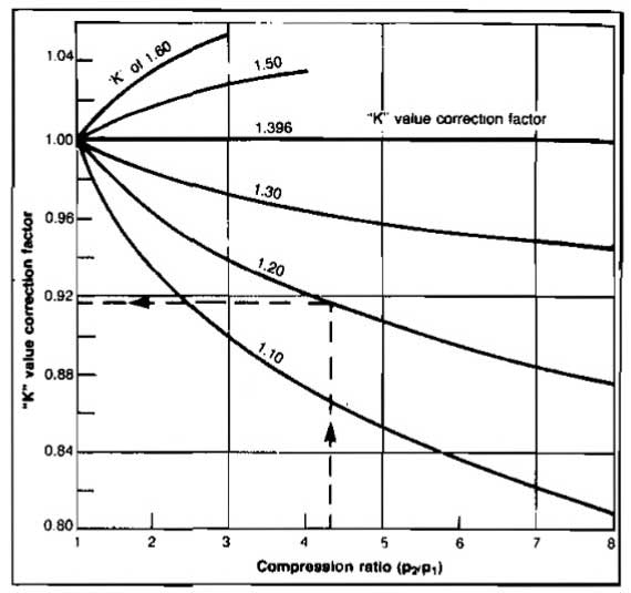
(K_corr) – is obtained from Picture 24;
p₁ – suction pressure, psia;
$\bar{Z}$
– average Z factor, and;
Z₁ – Z factor at p₁, T₁.

The number of stages required for a centrifugal compressor may be estimated from:

N = \frac{(BASIC HEAD) (K_{c o r r}) (28, 95) Z}{M (9 500)}

where:

N – number of stages;
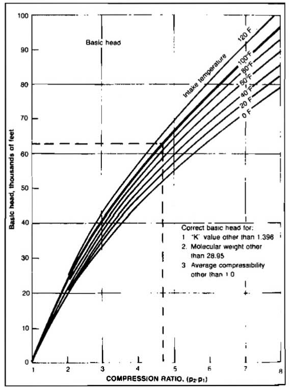
(BASIC HEAD) – is obtained from Picture 25;
(K_corr) – is obtained from Picture 24;
$\bar{Z}$
– average Z factor, and;
M – molecular weight of the gas.

Example 6:

Re-work Example 5 using Picture 23 and Picture 24. Also, estimate the number of stages required and the approximate compressor speed using Picture 25 and Picture 26.

Solution:

From Picture 23, for an intake volume of 4 550 ft³/min, the basic bhp ≈ 720 for a compression ratio of 4. From Picture 24, for a k value of 1,28 the k value correction factor is 0,956 for r = 4. Therefore:

bhp = \frac{720 (0, 956) (100) (0, 99)}{14, 5 (0, 988)} = 4 757 HP .

In order to estimate the number of stages required, from Picture 25, for:

r = 4 and;
T₁ = 80 °F;
Basic head ≈ 53 000 ft.

The number of stages is then:

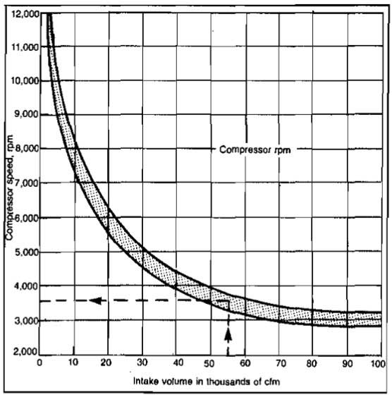
N = \frac{(53 000) (0, 956) (28, 95) (0, 99)}{17, 38 (9 500)} = 8, 9

This indicates that 9 stages will be required. The compressor speed is estimated by entering Picture 26 at an intake volume of 4 550 ft³/min and reading the speed as 9 800 rpm.

Footnotes