The liquefied natural gas (LNG) business has witnessed significant growth and transformation over the years, particularly in the realm of maritime transportation. LNG, a cleaner alternative to traditional fossil fuels, has gained traction as a primary energy source due to its lower emissions and abundance. With the increasing demand for LNG across various sectors such as power generation, transportation, and industrial applications, the need for efficient and reliable transportation methods has become paramount.
- LNG Business and history of ABS involvement with gas transportation at sea
- World Energy Demand
- Energy transporation-ships versus pipelines
- Natural gas exporting countries
- Natural Gas Importing Countries
- The Increase of Natural Gas Demand
- Costs and other Considerations
- Rate of Increase of the LNGC Fleet
- Comparison Between LNG and Oil
- Conversion Factors
- Cost of LNG
- ABS Experience with LNG Carriers
- Early Developments
- Further Developments
- Recent Acquisitions
- The ABS LNGC Fleet
ABS (American Bureau of Shipping) has played a pivotal role in shaping the history of gas transportation at sea. As a leading classification society, ABS has been involved in setting standards and regulations for LNG carriers and gas-related infrastructure, ensuring safety, reliability, and environmental protection. Since the inception of LNG transportation, ABS has been at the forefront of developing rules and guidelines for the design, construction, and operation of LNG carriers, contributing to the safe and efficient transportation of LNG cargoes worldwide. Through its technical expertise and industry collaboration, ABS continues to drive innovation and excellence in the LNG shipping sector, facilitating the expansion of LNG trade and the growth of the global energy market.
LNG Business and history of ABS involvement with gas transportation at sea
World Energy Demand
The following diagrams are intended to show energy demand and in particular how it is changing the supply ratios of commercially available sources of energy.
Figure 1 represents how world energy was produced in 2003.
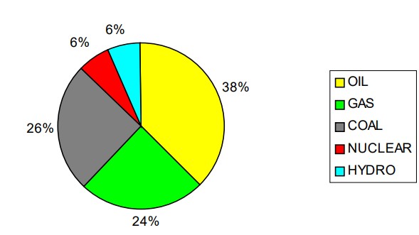
If we draw another pie diagram relative to the world energy production in 1991, we would get a very similar figure with only slight differences:
- oil 40 %,
- gas 23 %,
- coal 28 %,
- nuclear 7 %,
- and hydro 2 %.
It would seem that production changes in 12 years have been quite insignificant. However, considering the very large figures involved in the total world produced energy, even a variation of 1 percent is noticeable. The above figures clearly show that there is a clear trend of increase of the “clean” sources of energy (gas and water) and a decrease of the “dirty” sources (oil and coal), while the nuclear remains almost constant. This trend appears more evident comparing the rate of increase of the world energy consumption with the rate of increase of the various types of fuels for the 12 years period between 1991 and 2002. These rates of growth are indicated in Figures 2 and 3.
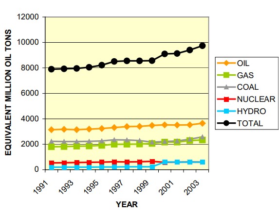
The diagram in Figure 3 is identical to that in Figure 2, except that total energy production line has been eliminated to magnify the differences between demand growths of the various energy sources.
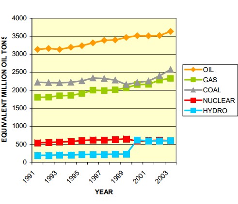
Table 1 shows the percentages of the total increase of energy demand and increases of the various sources from 1991 to 2002.
| Table 1. Increase of Energy Demand between 1991 and 2002 | |||
|---|---|---|---|
| Energy source type | Percentage (1991) | Percentage (2002) | Percentage increase between (1991-2002) |
| Total | 100 % | 100 % | 19,1 % |
| Oil | 40 % | 38 % | 12,4 % |
| Gas | 23 % | 24 % | 26,4 % |
| Coal | 28 % | 26 % | 7,8 % |
| Nuclear | 7 % | 6 % | 12,9 % |
| Hydro | 2 % | 6 % | 305 % |
Table 1 clearly shows that oil and coal percentages have decreased slightly, whilst the demand percentage for natural gas increased. Percentages relative to the growth of nuclear and hydro-electric sources, even though significant (especially the 300 % increase of the hydro-electric energy), are relatively small when compared to those produced by oil, gas and coal.
Energy transporation-ships versus pipelines
Natural gas exporting countries
Up to 1970, almost all natural gas was transported from the producing countries to the consuming countries via pipelines.
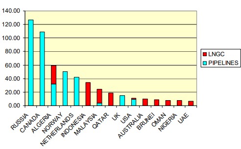
Pipelines are still used to transport the majority of natural gas today, particularly in Europe and United States. Table 2 indicates Planning the Design, Construction and Operation of New LNG Transportation Systemsnatural gas exporting countries, client countries and how the gas is shipped (e. g. by pipeline or by LNG carriers). The data in Table 2 are relative to the year 2002. The table is also useful to give an idea of the dimensions, the trends, the routes of gas and LNG in the world.
| Table 2. Natural Gas Exporting Countries | ||||
|---|---|---|---|---|
| Exporting Country | Importing Countries | Exported Volume (Billion of m3) | ||
| Pipeline | LNGC | Pipeline | LNGC | |
| Algeria | Italy, Portugal, Slovenia, Spain, Tunisia | Belgium, France, Italy, Spain, Turkey, USA | 32,15 | 26,88 |
| Argentina | Brazil, Chile, Uruguay | 5,17 | ||
| Australia | Japan, South Korea, Spain | 10,03 | ||
| Bolivia | Brazil | 2,50 | ||
| Brunei | Japan, South Korea, Spain | 9,07 | ||
| Canada | USA | 109,02 | ||
| Denmark | Germany, Sweden | 3,10 | ||
| France | Hungary, Switzerland | 1,20 | ||
| Germany | Australia, Belgium, Hungary, Luxemburg, Poland, Romania, Switzerland | 4,48 | ||
| Indonesia | Japan, South Korea, Taiwan | 34,33 | ||
| Lybia | Spain | 0,63 | ||
| Malaysia | Singapore, Thailand | Japan, South Korea, Taiwan, USA | 4,00 | 20,52 |
| Mexico | USA | 0,05 | ||
| Netherlands | Belgium, France, Germany, Italy, Luxemburg, switzerland | 42,20 | ||
| Nigeria | France, Italy, Portugal, Spain, Turkey,USA | 7,84 | ||
| Norway | Australia, Belgium, Czech Republic, France, Germany, Italy, Netherlands, Poland, Spain, UK | 50,60 | ||
| Oman | France, Japan, South Korea, Spain, USA | 7,98 | ||
| Qatar | Japan, South Korea, Spain, USA | 18,59 | ||
| Russia | Australia, Bulgaria, Croatia, Czech Republic, Finland, France, Germany, Greece, Hungary, Italy, Netherlands, Poland, Spain, Romania, Slovakia, Slovenia, Switzerland, Turkey, Others | 126,86 | ||
| Trinidad&Tobaco | Puerto Rico, Spain, USA | 5,32 | ||
| Turkmenistan | Iran | 4,20 | ||
| UAE | Belgium, Japan, South Korea, Spain | 6,85 | ||
| UK | Belgium, France, Germany, Ireland, Netherlands | 15,08 | ||
| USA | Canada, Mexico | Japan | 9,15 | 1,7 |
| Total | 411,32 | 148,99 | ||
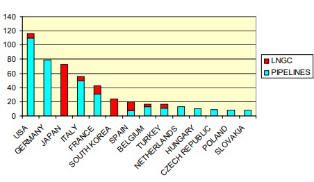
From Table 2 it appears that in 2002, 73 % of the exported gas had been transported via pipelines, while only 27 % has been shipped by sea transportation. Figure 4 indicates the share of exported natural gas among the first 15 exporting countries.
Natural Gas Importing Countries
From the point of view of the importers, Table 3 indicates for each importing country how much gas has been imported through pipelines and how much has been imported through ships. Both Tables 2 and 3 are to be read taking into account that some countries may appear as importer because the gas is delivered in terminals situated in their territory and as exporter as the imported gas is then shipped to other countries through pipelines.
| Table 3. Natural Gas Importing Countries | |||
|---|---|---|---|
| Importing Countries | Imported Volume (Billion of m3) | ||
| Pipeline | LNGC | Total | |
| Australia | 6,04 | 6,04 | |
| Belgium | 13,22 | 3,30 | 16,52 |
| Brazil | 3,00 | 3,00 | |
| Canada | 4,87 | 4,87 | |
| Chile | 4,60 | 4,60 | |
| Croatia | 1,08 | 1,08 | |
| Czech Republic | 9,20 | 9,20 | |
| Finland | 4,34 | 4,34 | |
| France | 31,14 | 11,54 | 42,68 |
| Germany | 78,75 | 78,75 | |
| Greece | 1,48 | 0,50 | 1,98 |
| Hungary | 9,97 | 9,97 | |
| Iran | 4,20 | 4,20 | |
| Ireland | 3,42 | 3,42 | |
| Italy | 49,55 | 5,70 | 55,25 |
| Japan | 72,69 | 72,65 | |
| Luxemburg | 0,80 | 0,80 | |
| Mexico | 4,28 | 4,28 | |
| Netherlands | 13,13 | 13,13 | |
| Poland | 8,40 | 8,40 | |
| Portugal | 2,20 | 0,43 | 2,63 |
| Puerto Rico | 0,63 | 0,63 | |
| Romania | 3,00 | 3,00 | |
| Singapore | 2,50 | 2,50 | |
| Slovakia | 7,90 | 7,90 | |
| Slovenia | 1,04 | 1,04 | |
| South Korea | 23,91 | 23,91 | |
| Spain | 7,76 | 12,28 | 20,04 |
| Sweden | 0,90 | 0,90 | |
| Switzerland | 3,05 | 3,05 | |
| Taiwan | 7,00 | 7,00 | |
| Thailand | 1,75 | 1,75 | |
| Tunisia | 1,20 | 1,20 | |
| Turkey | 11,04 | 5,35 | 16,39 |
| UK | 2,70 | 2,70 | |
| Uruguay | 0,07 | 0,07 | |
| USA | 109,67 | 6,41 | 116,08 |
Figure 5 indicates the share of imported natural gas among the first 15 largest importing countries.
The Increase of Natural Gas Demand
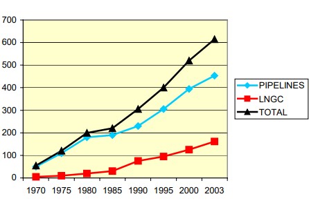
Figures 6 and 7 indicate how the transportation of gas has increased for the last thirty years, since the appearance of the first LNG carriers (late fifties) and continuing up to the end of 2002. Both Figures show in a different graphic view the increase of gas transported through pipelines, International trade of Liquefied Natural Gas in maritime industryLNG transported by sea and total gas exported.
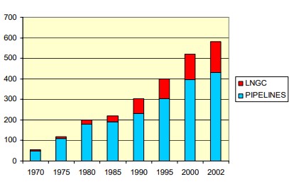
It is interesting to note that the slope of the curve representing the Natural Gas Transportation in the Form of Hydrate Pellets (NGHP)LNG transported by sea (the red line) in Figure 7 reaches its maximum in the period between 2000 and 2003, even though this period is shorter than the other periods considered in the diagram that are five-year intervals.
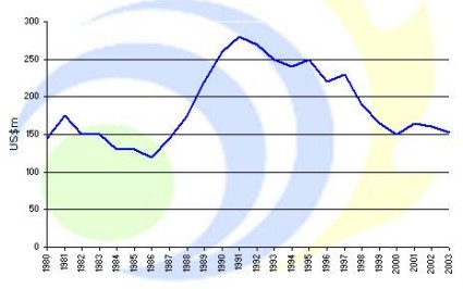
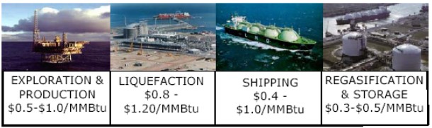
Costs and other Considerations
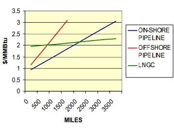
Figure 8 shows a rough comparison among the difference of cost of gas to the power stations depending on the means used for its transport. It is shown that as the distance between the gas exporter and the importer increases, transportation by LNG carriers becomes more cost effective. In general, transportation by sea (including the cost of ships, terminals gas liquefaction at the exporting terminal and LNG gasification at the importing terminal) becomes non cost effective for distances of about 700 miles and above with respect to offshore pipelines and approximately 2 200 miles and above with respect to on-shore pipelines.
It can be noted that there is tendency of the intersections of the lines in Figure 8 moving towards left. Considering that the cost of LNG is made by the sum of the costs of the four steps of the so-called “LNG chain“, this trend depends from the reduction of the cost of the various parts of the chain:
- Exploration and production.
- Liquefaction.
- Transportation by sea.
- Re-gasification and storage.
In particular the cost of the LNG carriers reduced significantly during the last twenty years, as indicated in the following Figure 9.
Moreover, considering cargo carrying capacity increases of future ships, the associated reduction of the transportation cost of LNG, the use of ships for worldwide gas transportation will continue to increase.
Ships, in fact, provide numerous advantages compared to pipelines, which are difficult to translate to financial terms, but still represent a considerable economic advantage. The main advantages are the following:
- Pipelines, once constructed from exporting country to importing country restrict future flexibility of new markets for the product. Both countries are bound together until new expensive pipelines are built.
- Pipelines are much more exposed to natural disasters, political disputes and even terrorist attacks than ships.
- Long pipelines cross many different countries. Royalties are to be paid to each country crossed that may increase the requested royalties at any time blackmailing both the exporter and the final importer.
- The new gas exporting countries are situated very far from the importing countries.
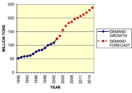
All market analysts forecast a continuous growth of LNG demand in the foreseeable future. Figure 10 shows the growth of LNG demand from 1990 to 2003 and then its extrapolation up to 2015.
Rate of Increase of the LNGC Fleet
The first LNG carriers were built in the late 1960’s. Since the first ships started to operate successfully, there was a large increase the number of ships and cargo carrying capacity until the 1980’s. After this period, there was decreased interest on the transportation by sea versus transportation by pipeline.
Many of the existing LNG carriers were laid up for long periods. In the middle of the 1990’s, the emergence of new exporting countries far from importing countries, development of favorable political situation, reduced cost of LNG carriers, very good safety records of the existing LNG carriers and the construction of new terminals reversed the previous trend and started a tremendous increase of LNG carriers construction. Figure 11 shows this increase from 1970 to 2003 in five-year intervals. The last portion of the line (between 2000 and 2003) being the period of considered time reduced with respect to
the previous periods, may give a wrong impression, therefore, it has been also indicated the projection to 2005.
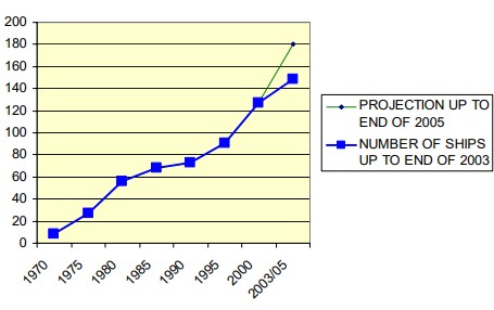
Considering the total cargo carrying capacity of the LNG worldwide fleet (instead of only the number of ships) it becomes possible to draw a diagram with a trend almost identical to the trend of Figure 9, starting from a total cargo carrying capacity of about 350 000 m3 at the end of 1970, arriving to about 17 300 000 m3 at the end of 2003.
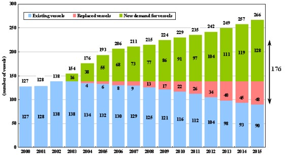
Finally, Figure 12 shows a projection up to 2015 of the LNG carriers that will be necessary to transport the quantities of LNG as indicated in Figure 10 (by year).
Comparison Between LNG and Oil
Conversion Factors
Different types of fuels may be compared by considering the different quantities of energy generated by a unit of each of the different fuels. This is done by comparing the amount of fuel necessary to generate a comparable unit of energy. In general the most used energy unit is the BTU 1 BTU (British Thermal Unit) is the amount of heat (energy) required to raise the temperature of 1 pound of water by 1 °F. BTU is equal to 0.252 kcal, being 1 kcal the amount of heat required to raise the temperature of 1 kg of water by 1 °Cx: it is therefore possible to compare LNG and crude oil making reference to this unit, or better, as this unit is quite small, to 1 million of BTU As an order of magnitude, 1 million BTU is the energy necessary to produce in a modern power station about 300 kW-h x.
Table 4 gives a number of conversion factor that can be used to make a comparison between, for instance, the potential energy transported by a tanker and a LNGC.
| Table 4. Energy Conversion Factors | |||||||
|---|---|---|---|---|---|---|---|
| Millions BTU | Bbls of Oil equivalent | Tons of Oil equivalent | Cu.ft Gas | Cu.m Gas | 1 Cu.m LNG | 1 Ton LNG (SG = 0,45) | |
| 1 Million BTU | 0,172 | 0,0235 | 1 | 28,3 | 0,0459 | 0,0206 | |
| 1 Bbl of Oil equivalent | 5,8 | 0,136 | 5,8 | 164,2 | 0,266 | 0,1195 | |
| 1 Ton of Oil equivalent | 42,5 | 7,33 | 42,5 | 1200 | 1,95 | 0,8765 | |
| 1 Cu.ft Gas | 0,001 | 0,000172 | 0,0000235 | 0,0283 | 0,0000458 | 0,0000206 | |
| 1 Cu.m Gas | 0,0353 | 0,000608 | 0,000830 | 35,3 | 0,00162 | 0,000742 | |
| 1 Cu.m LNG | 21,8 | 3,76 | 0,513 | 21,824 | 618 | 0,45 | |
| 1 Ton LNG (SG=0,45) | 48,6 | 8,38 | 1,144 | 48,65 | 1375 | 2,229 | |
From the data in Table 4, it would appear that the potential energy transported by a 145 000 m3 LNGC is nearly equivalent to the potential energy transported by a 75 000 DWT oil tanker.
Cost of LNG
Figure 13 indicates how the four steps of the LNG chain contribute to the cost of LNG necessary to produce one million BTU.
From the values indicated in Figure 13, it would appear that the “net” cost of LNG would be in the range between 2 to 3,7 Us Dollars per Million BTU. The cost of transportation to the power station and the cost of energy production are to be added.
In general, the actual cost of the gas obtained from LNG at an US power station (all included) necessary to produce 1 million BTU ranges between 4,5 and 5,5 USD, this figure being almost equivalent to the cost of the oil necessary to produce the same amount of energy.
ABS Experience with LNG Carriers
Early Developments
ABS has been involved with the development of LNG marine transportation technology as early as 1953. Since the classification of the first LNG carrier “METHANE PIONEER” in 1958, ABS has been in the forefront of LNG technology.
During the 1960’s and early 1970’s ABS classed 11 LNGC of various configurations with cargo capacity ranging from 27 400 m3 (“METHANE PRINCESS” and “METHANE PROGRESS” to 71 500 m3 (“POLAR ALASKA” and “ARTIC TOKYO“). During the same period there was much work being done on international level in the development of what eventually become the International “Code for the Construction and Equipment of Ships Carrying Liquefied Gases in Bulk” (IGC Code). ABS participated in these efforts with other Classification Societies in the IACS Gas Carrier Committee. This Group developed criteria for design, construction and surveys, which were submitted for consideration to IMO. ABS, being the most experienced Classification Society on gas carriers, played a major role in this effort.
Read also: Natural Gas Transportation in the Form of Hydrate Pellets (NGHP)
At the same time the USCG formed the Chemical Transportation Advisory Committee (CTIAC) to help to formulate a U.S. position for the deliberations at IMO. ABS was invited to be one of the eight original members of this group and remained fully participatory serving in an advisory capacity to the USCG throughout the development of the IGC Code.
Further Developments
The ten 126 000 m3 vessels built at General Dynamics with spherical aluminum tanks were the first such vessels built in that yard. ABS involvement in that project began on early 1972 with a conceptual review of the Moss-Rosenberg containment system design. ABS conducted independent sea-keeping analysis, 3-D and detailed 2-D FEM analysis and vibration analysis. ABS surveyors attended and supervised welder and welding procedure qualifications at the tankfabrication site in South Carolina while the fabricator was developing the procedures and the techniques for the fabrication of the aluminum tanks.
Over a period of several years completed tanks supported at the equatorial rings were being transported by barges from South Carolina to Quincy, Massachusetts, and installed in the vessels at the rate of one tank per month. This required an extensive coordination and project management on the part of ABS.
The three 125 000 m3 LNG vessels using the Technigaz MARK 1 membrane system were built at Newport News to ABS Class for El Paso. This construction was handled by the same technical staff and concurrently with the review of the above-described project at General Dynamics.
In the early 1980’s five 130 000 m3 LNG vessels using the Gaz Transport membrane cargo containment system were constructed in two French shipyards (3 at Societe’. Metal and Navale, Dunkerque and 2 at Constructions Navales and Industrielles De la Mediterranee, La Seyne) and delivered over a two years time frame to Malaysia International Shipping Corporation (MISC). The plan review for these ships was performed by the ABS London Engineering Office.
Recent Acquisitions
In the early 1990’s, ABS classed the first two LNGC built incorporating the IHI prismatic type B cargo containment system. These vessels of 87 500 m3 carrying capacity were constructed at IHI’s yard of Chiba, Japan for Phillips Marathon.
ABS then classed the first two LNGC with membrane type cargo containment system (Gaz Transport system) built in Italy for SNAM (the shipping Company of ENI, the National Italian Oil Company). ABS organized a one-week full immersion seminar for its Surveyors,also attended by shipyard and owner’s representatives who did not yet have previous experience.
Ten more 135 000 m3 LNG carriers with Moss-Rosenberg cargo containment system were built at three Japanese shipyards: MHI, MHE and KHI under NK class. Qatar Liquefied Gas Corp., the charterer of these ships, appointed ABS Marine Services to carry out plan review and supervision during construction on their behalf. All drawings relative to cargo containment and cargo handling system, hull structure, machinery and electrical systems were reviewed by ABS Yokohama Office. The analyses reviewed by ABS included hull FEM analysis, cargo tank and skirts FEM analysis, buckling and fatigue crack propagation analysis and heat transfer calculation for selection of hull materials.
In 1997, ABS Engineering assisted Samsung Heavy industries (SHI) to develop drawings for the first 135 000 m3 LNGC built by the shipyard, which led to SHI becoming a world leader in LNGC construction.That ship was also the first vessel of this size to use the MARK III membrane cargo containment system. This system, developed by Technigaz, was previously used only for two 18 500 m3 ships built in Japan. This first ship, “SK SUPREME“, was followed by five other ships built at SHI. Presently ABS has orders for other 22 ships ranging from 138 000 to 155 000 m3 to be built at SHI, DSME, Japan and China.
Currently, ABS is involved in the review and approval of the concept designs for new generations of LNGC with cargo carrying capacity ranging from 205 000 to 250 000 m3 .
ABS is the only Classification Society to have classed ship with all types of cargo containment system, which have been used to date.
The ABS LNGC Fleet
Table 5 is the list of all LNGC ships built with ABS class up this date.
| Table 5. LNGC‘s built with ABS Class | ||||||
|---|---|---|---|---|---|---|
| Ship Name | Shipyard | Year | Capacity (m3) | Cont.Nt System | Materials | |
| 1 | Methane Pioneer | Alabama DD&SB Co. | 1958 | 5,123 | Prismatic free standing | Aluminum |
| 2 | Methane Princess | Vickers-Armstrong | 1964 | 27,400 | Prismatic (Conch) | Aluminum |
| 3 | Methane Progress | Harland & Wolf | 1964 | 27,400 | Prismatic (Conch) | Aluminum |
| 4 | Methane Arctic | Kockums | 1969 | 71,500 | Membrane (Gas Transport) | Invar |
| 5 | LNG Palmaria | Italcantieri | 1969 | 40,000 | Prismatic (Esso) | Aluminum |
| 6 | Mathane Polar | Kockums | 1969 | 71,5000 | Membrane (Gaz Transport) | Invar |
| 7 | LNG Elba | Italcantieri | 1970 | 40,000 | Prismatic (Esso) | Aluminum |
| 8 | Esso Porto Venere | Italcantieri | 1970 | 40,000 | Prismatic (Esso) | Aluminum |
| 9 | Laieta | Astilleros y Talleres del Noroeste | 1970 | 40,000 | Prismatic (Esso) | Aluminum |
| 10 | Descartes | Chantier de l’Atlantique | 1971 | 40,000 | Membrane (Technigas Mark1) | Stainless Steel |
| 11 | Massachussets | Todd Shipyard | 1973 | 5,000 | Cylindrical Free Standing tanks | Aluminum |
| 12 | Isabella | Construction Navales et Industrielles de la Mediterranee | 1974 | 35,000 | Membrane (Gas Transport) | Invar |
| 13 | LNG Aquarius | General Dynamics | 1977 | 126,000 | Moss-Moss-Rosenberg | Aluminum |
| 14 | LNG Aires | General Dynamics | 1978 | 126,000 | Moss-Moss-Rosenberg | Aluminum |
| 15 | LNG Capricorn | General Dynamics | 1978 | 126,000 | Moss-Moss-Rosenberg | Aluminum |
| 16 | LNG Gemini | General Dynamics | 1978 | 126,000 | Moss-Moss-Rosenberg | Aluminum |
| 17 | LNG Leo | Gereral Dynamics | 1978 | 126,000 | Moss-Moss-Rosenberg | Aluminum |
| 18 | LNG Libra | General Dynamics | 1979 | 126,000 | Moss-Moss-Rosenberg | Aluminum |
| 19 | LNG Taurus | General Dynamics | 1979 | 126,000 | Moss-Moss-Rosenberg | Aluminum |
| 20 | LNG Vigro | General Dynamics | 1979 | 126,000 | Moss-Moss-Rosenberg | Aluminum |
| 21 | LNG Edo | General Dynamics | 1980 | 126,000 | Moss-Moss-Rosenberg | Aluminum |
| 22 | LNG Abuja | General Dynamics | 1980 | 126,000 | Moss-Moss-Rosenberg | Aluminum |
| 23 | El Paso Paul Kayser | Soc.Metal et Navale,Dunkeque | 1975 | 125,000 | Membrabe (Gas Transport) | Invar |
| 24 | El Paso Sonatrach | Soc.Metal et Navale,Dunkeque | 1978 | 125,000 | Membrane (Gas Transport) | Invar |
| 25 | El Paso Consolidated | Soc. Metal et Navale,Dunkeque | 1978 | 125,000 | Membrane (Gas Transport) | Invar |
| 26 | Edouard L.D. | Soc. Metal et Navale,Dunkeque | 1977 | 125,000 | Membrane(Gas Transport) | Invar |
| 27 | Tenaga Tiga | Soc. Metal et Navale,Dunkeque | 1981 | 130,000 | Membrane (Gas Transport) | Invar |
| 28 | Tenaga Dua | Soc.Metal et Navale,Dunkeque | 1981 | 130,000 | Membrane (Gas Transport) | Invar |
| 29 | Tenaga Satu | Soc. Metal et Navale, Dunkeque | 1982 | 125,000 | Membrane(Gas Transport) | Invar |
| 30 | Tenaga Lima | Costr.Navales de la Meditarranee | 1981 | 138,000 | Membrane (Gas Transport) | Invar |
| 31 | Tenaga Empat | Costr.Navales de la Meditarranee | 1981 | 130,000 | Membrane (Gas Transport) | Invar |
| 32 | LNG Delta | Newport News | 1978 | 125,00 | Membrane (Technigas Mark I) | Stainless steel |
| 33 | Galeomma | Newport News | 1978 | 125,000 | Membrane (Technigas Mark I) | Stainless steel |
| 34 | Matthew | Newport News | 1979 | 125,000 | Membrane (Technigas Mark I) | Stainless steel |
| 35 | LNG Bonny | Kockums | 1981 | 133,000 | Membrane (Gas Transport) | Invar |
| 36 | LNG Finima | Kockums | 1984 | 133,000 | Membrane (Gas Transport) | Invar |
| 37 | Polar Eagle | IHI | 1993 | 87,500 | Prismatic (IHI SBP) | Aluminum |
| 38 | Arctic Sun | IHI | 1993 | 87,500 | Prismatic (IHI SBP) | Aluminum |
| 39 | LNG Porto Venere | Sestri Cantiere Navale | 1995 | 65,700 | Membrane (Gas Transport) | Invar |
| 40 | LNG Lerici | Sestri Cantiere Navale | 1998 | 65,700 | Membrane (Gas Transport) | Invar |
| 41 | SK Supreme | SHI | 1999 | 138,000 | Membrane (Technigas Mark III) | Stainless steel |
| 42 | SK Splendor | SHI | 2000 | 138,000 | Membrane (Technigas Mark III) | Stainless steel |
| 43 | SK Stellar | SHI | 2000 | 138,000 | Membrane (Technigas Mark III) | Stainless steel |
| 44 | SK Sunrise | SHI | 2003 | 138,000 | Membrane (Technigas Mark III) | Stainless steel |
| 45 | Fuwairit | SHI | 2003 | 138,000 | Membrane (Technigas Mark III) | Stainless steel |
The diagram in Figure 14 depicts classification of LNG carriers at new construction yards. This diagram does not take into account possible changes of class of existing ships.
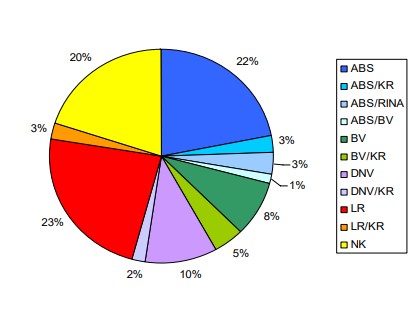
As a number of ships have dual class, Table 6 shows the actual percentages of the ships built under each Classification Society. This being the case, the sum of the percentages in Table is greater than 100.
| Table 6. Percentage of LNG’s Built under Various Classes | |
|---|---|
| Classification Society | Percentage of LNGC‘s |
| ABS | 29 % |
| LR | 26 % |
| NK | 20 % |
| BV | 13 % |
| KR | 13 % |
| DNV | 12 % |
| RINA | 3 % |