Dynamic simulation and optimization of LNG Plants has established itself as a valuable technology in the chemical process industries. Both steady state and dynamic simulation are carried out in the various stages of the process life cycle. These models are useful for a variety of purposes, including but not limited to engineering and process studies, control system studies, and applications in day-to-day operations. Improvements in usability of the dynamic simulation software tools and the innovations in computing technology have led to the further deployment and novel applications of process simulation tools. The operability and profitability of the plant during its life depends on good process and control system design. Dynamic simulation helps to ensure that these aspects are analyzed early in the plant design stage. This helps to eliminate any costly rework that may be needed later.
- Introduction
- Life cycle dynamic simulation of LNG plants and import terminals
- Dynamic modeling of LNG plants
- Differences from steady state modeling
- Dynamic modeling of individual equipment in LNG plants
- Fidelity and details in LNG plant dynamic models
- Applications of dynamic simulation in LNG
- LNG process design studies
- Compressor antisurge system design
- Operability and controllability analysis
- LNG plant startup simulations
- Dynamic optimization of LNG plant design
- Relief system design and safety scenarios
- Plant troubleshooting and operational support
- Plant production enhancements and debottlenecking
- Control system checkout
- Operator training simulator
- Advanced process control development
- Dynamic simulation of LNG import terminals
- Dynamic modeling of LNG import terminals
- Applications of dynamic simulation in LNG import terminals
- Case study: LNG import terminal dynamic simulation
Introduction
In the early days of its development, dynamic simulation was used for very specialized applications, mainly due to the lack of user-friendly software applications. These tools required custom development and hence, were not widely deployed. Gradually, the usability of dynamic simulation tools improved over the years. The availability of software packages with built-in unit operation models and physical property packages that can easily be utilized to put together plantwide dynamic models made the application of this technology widely accepted.
In the beginning, the main application of dynamic models was for development of operator training simulators. These models were not necessarily of high fidelity, but were computationally simpler. Since the 1990s, software applications that are easy to use and based on rigorous thermodynamics have entered the market. These made the application of dynamic simulation more widespread. Another very important factor was the increase in computational power that became readily available over the years. With Moore’s law becoming a reality, computational capabilities have gone up significantly over time. This made the application of detailed, plantwide high fidelity dynamic models more feasible.
Several benefits can be realized by using the dynamic simulation in the various stages of an LNG plant life cycle. These include both design and operational benefits. On the process design side, it is an important tool for evaluating the antisurge control system for the refrigeration compressors and sizing the antisurge valves. The reliable protection of this key equipment is critical for reliable long-term operation of the LNG plant. Also, dynamic simulation can be pivotal in the sizing of specific key relief valves, and the overall relief system and optimum selection of equipment sizes. LNG plants are also characterized by extensive heat integration, the operational implications of which can be verified by simulation. Further, the effect of external factors like ambient conditions and compositional changes on the future plant operation can be analyzed to further optimize the design. The startup procedures can be developed or verified before any field activities, thus potentially saving valuable startup time.
On the control system side, dynamic simulation can help to ensure that the plant has sufficient design margins to handle the disturbances. Also, dynamic simulation can be used to assess the optimal operation of the LNG plant in the face of changing conditions like ambient temperature. There is a greater emphasis now on considering plant operability in the design stage. Plantwide dynamic models along with operability metrics are valuable tools in attaining this objective. A dynamic simulation model of the LNG plant can also be used for the checkout of the plant distributed control system (DCS) prior to commissioning. This helps to reduce the time needed for commissioning on-site during startup. Also, this simulation model can be leveraged for startup support and for operator training purposes. The direct and indirect benefits of these applications are many, including better plant startup, less plant downtime, and improved safety.
Dynamic simulation has found wide applicability in the LNG industry. The various engineering contractors have used dynamic simulation extensively for improving the plant design. Also, process licensors have used these tools to improve and optimize their offerings. Apart from these, the LNG plant owner-operators have also found good use of dynamic simulation, especially in the form of operator training simulators.
The chapter starts with a brief overview of life cycle dynamic simulation of LNG plants. The details of developing LNG plant dynamic models, including the modeling of individual unit operations, is presented. The applications of dynamic simulation in LNG plants, including engineering studies and operator training simulator (OTS) are also presented in this chapter. In addition, the development of dynamic models and their applications in design and operation of LNG import terminals is discussed here.
Life cycle dynamic simulation of LNG plants and import terminals
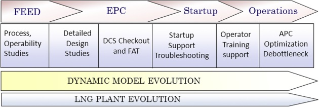
Dynamic simulation analysis is used in the various stages of plant life cycle for different applications. The benefits of integrating these modeling activities have been realized over the years. This has led to the adoption of life cycle modeling concepts by various process-engineering companies and the vendors of simulation tools. The dynamic model, evolving with the various stages of a plant life cycle, can be tailored for various applications within the project life cycle (Figure 1). A brief description of the main project stages are given next.
- Process Studies. There are many nonproject-specific studies that utilize the benefits of dynamic analysis and investigate the potential for LNG process design improvement. These are aimed at improving the process design rather than a specific plant design. An example is the study of plantwide control structure for the LNG process using a base dynamic model;
- FEED. The Front End Engineering and Design (FEED) stage is characterized mainly by steady state information about the plant. Some of the more detailed information pertinent to dynamic simulation is not available at this stage. For example, equipment and control valve sizes and pressure profiles are not fixed. Dynamic simulation can still be a valuable tool in making qualitative decisions in this stage. The ability to influence the LNG project is highest in the FEED phase, while the cost committed is the lowest. Operability studies that look at the specific plant can be done here. For these studies, a certain level of uncertainty can be accommodated in decision-making;
- EPC. The detailed design of the LNG plant is performed in the Engineering, Procurement, and Construction (EPC) stage. The equipment and line sizes, isometric layout, and other details are available at the end of the EPC stage, as issued for construction. This makes the EPC stage a suitable phase for development of high fidelity dynamic models. Engineering studies and control system checkout studies can be carried out efficiently in this stage. The dynamic model that is plant-specific is best developed at the EPC stage of the project. The engineering studies model may easily be extended to a fully functional virtual plant/OTS at this stage;
- Startup/Commissioning and Operations. The startup and commissioning activity involves bringing the LNG plant to normal operation and completing a subsequent performance test of the plant before turnover to the operating firm. This includes a commissioning test for the individual units and a performance test for the overall facility. Dynamic simulation can be valuable in various startup studies, operator training, and additional on-site control system checkout studies in this stage. The model at this stage would have all the details pertinent to the as-constructed plant. The model can then be utilized for troubleshooting and operational support throughout the plant life cycle.
Dynamic modeling of LNG plants
A dynamic simulation model that is fundamental and based on rigorous thermodynamics is the preferred option for simulation analysis. The scope, level of detail, and fidelity of the model can be tailored to suit the application it is used for and the amount of information available for modeling. Several commercially available simulation packages can be utilized for developing dynamic simulation models for LNG plants. Different software packages have different strengths and capabilities. The selection of the right software needs to be based on the user preference and the scope and type of the study. For example, in certain cases, detailed hydraulic capabilities may be required in the model. These applications may need the use of software beyond the standard lumped volume modeling tools in the market. It is also possible to interface different software packages with different capabilities to enhance the overall applicability of the simulation. A good example is the use of OLGA or other upstream hydraulic models with process simulation tools, which enables modeling of scenarios like slugging in the gas pipelines feeding the LNG plant. It is beneficial to integrate the models for upstream pipelines to the LNG plant dynamic model in this case.
Differences from steady state modeling
The main advantage of using dynamic simulation is the ability to capture the time-dependent behavior of the system. This functionality comes at the price of increased data and resource requirements. Unlike steady state simulation, dynamic simulation is characterized by the need for accurate pressure profile, equipment volume, and other relevant information. Hence, the amount of information required for a high fidelity dynamic simulation is significantly more compared to steady state models. The internal variable specifications for dynamic simulation are much less. Normally, only the boundary conditions like pressure and temperature need to be specified and almost all the internal variables are calculated. Steady state simulation, especially for conceptual design, allows one to specify many more variables internally.
A clear distinction needs to be made between models and simulation. Models are tools that are used for various purposes, simulation being one of them. There are several other applications for these models (such as optimization, state estimation, etc.). Hence, the dynamic models can be used for steady state simulation in certain special cases, where there is a need to evaluate only a few steady states. This is usually beneficial if a dynamic model is already available and can be leveraged for the intended purpose.
Dynamic modeling of individual equipment in LNG plants
This section describes the main components of the LNG plant dynamic model and the approaches that can be used for modeling this equipment. Different modeling approaches can be used depending on the fidelity desired and the computational resources available. These are explained in the following sections.
Piping
The exact modeling approach for the plant piping depends on the purpose of the dynamic model. For detailed engineering studies, accurate volume and pressure drop in the piping becomes important. In these cases, the detailed piping layout drawings or isometric drawings can be used to obtain the required information. For lumped volume simulation applications, the piping data may be condensed to lumped volumes and equivalent lengths or other similar input.
For applications where momentum balance equations in the pipe hydraulics are important, the models need to be developed with more detail. These models tend to be more specialized and limited to smaller sections of the plant. Simulation software packages in the market that are commonly used may not be suitable to handle these applications. An example of the application is analysis of pressure surge in pipelines and heat exchanger tube rupture simulations. Another important consideration in the modeling of piping is the ability to accurately model the choked flow in pipes. For applications that require the solution of momentum balance equations, extensions to the standard simulation tools or specialized hydraulic analysis software tools may be more appropriate.
Control and isolation valves
The specification of the control valve and isolation valve data is important for accurately capturing the dynamic responses in the model. The control valves are modeled using the actual valve size, char-acteristic, and the actuator timings. The valve size can be represented using rated Cv data from the vendor. For the characteristics, actual vendor characteristics need to be used. The speed of the actuator is also an important parameter in the simulation, since this determines the dynamic response of the overall control loop. This could be an input or can be determined from the simulation as a requirement to meet a specified dynamic response.
Further detailed modeling of valves involves using the actual valve sizing equations from the vendor. Some of the simulation software tools allow use of these in addition to the universal gas sizing equation. It is important to use the correct pressure differential ratio factor (Xt) and other vendorspecific parameters for the valve that may impact the sizing calculations in this case.
Compressors and pumps
Since LNG plant designs utilize refrigeration processes, compressor performance needs to be accurately captured for the fidelity of the plantwide simulation model. For dynamic modeling of compressors, the following items are important.
- A full performance curve is needed to accurately model compressors. These curves give compressor flow vs. head and flow vs. efficiency relationships at different speeds or Inlet Guide Vane (IGV) positions. The curves would preferably be as-tested curves in the field or final design curves. The full speed range from 0 to maximum operating speed is preferred for modeling. Since the vendor curves normally are limited to a certain set of speeds, extrapolation of the curves using fan laws may become necessary to capture the coast-down and startup behavior at lower speeds;
- Rotational inertia information to capture the effect of transient rotational power during startup, coast-down, and other dynamic events.
To enhance the model fidelity, it is possible to utilize multiple curves for different molecular weights or inlet conditions. Multiple molecular weight curves are useful for cases where compositions are expected to change. This may be more relevant for mixed refrigerant compressors with varying compositions and less for cascade processes with fixed refrigerant compositions. Multiple curves at different suction pressures would allow more accurate modeling for the cases where suction conditions vary significantly. This could be important for some detailed engineering studies.
In dynamic simulation, the operating point in the compressor map is determined based on the overall system hydraulic and other conditions. The variation in speed can be either modeled as an external specification or can be calculated by the compressor model based on the shaft power balance. If the speed variation is to be modeled, the rotational inertia of the compressor needs to be input into the model. The efficiency at the operating point is used to calculate the power consumption.
For accurate modeling of pumps, the pump characteristic curve is needed to model the head-flow relationship under different conditions. Since the pumps used are mostly fixed speed pumps, this usually is specified only at the operating speed.
Expanders
The expanders are utilized in the LNG plants to increase the efficiency and recover energy while reducing feed gas pressure. These could be vapor expanders or flashing liquid expanders. The modeling methodology for expanders is very similar to the compressors. Full performance curves (Figure 2) for the expanders can be utilized for modeling purposes. These expander curves would provide flow vs. head or flow vs. power relationships (and efficiency) at different expander speeds. This methodology is commonly used in the commercial simulation packages.

If the full curves are not available, the expander can be modeled with the expander flow equation. This is a typical resistance equation, whereby the conductance can be specified based on the flow and pressure drop based on the normal operating conditions. There should be provisions to consider choking in the expander in this case (as the flow would be limited and independent of the downstream pressure). The efficiency can be used along with the isentropic expansion equations to calculate the power generated in the expander.
Gas turbine drivers and electric motors
The refrigeration compressors in the LNG plant are mostly driven by gas turbines. In some cases, electric motors or steam turbines may be used as the drivers. The modeling of the gas turbine and the associated dynamics is useful to accurately capture the dynamic behavior of the LNG plant. Normally, the turbine governor speed controller resides in the gas turbine control package. The response of the turbine speed control and hence the power supply has an impact on the overall plant response.
There are two alternate routes to modeling the gas turbines, depending on the application of the model and the fidelity required. The first option is to build a fundamental model based on the com-bustion of the fuel with air and subsequent expansion. In this case, the air compressor needs to be modeled with actual curves to get the correct representation. Also, the combustion equations need to be modeled rigorously. The flue gas is fed to an expander, which generates the shaft power. The expander curves also have to be accurate to get the right relationship between speed, power, and flue gas exhaust temperature.
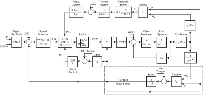
The approach to modeling a gas turbine with the combustion and expansion phenomena explained earlier is computationally demanding. This approach can also be challenging due to the lack of accurate data. This type of detailed model is not required for the LNG process related dynamic studies that are commonly performed. An alternative option is to use empirical models for the gas turbines. These models are based on transfer functions that capture the essential dynamics of the system. The various lags and delays in this model are used to represent the dynamics of the fuel gas positioner/ valve, fuel system, and the combustor.
An empirical model for the gas turbine reported by Rowen (1983) is shown in Figure 3. Here, the speed governor, fuel system, and valve positioner dynamics are represented by first order transfer functions. The shaft power is calculated based on the fuel flow and speed and used in the compressor model to denote shaft power. A balance between power supply and demand is used to compute turbine speed.
The modeling of the control schemes that are internal to the gas turbine can also be important. Apart from speed control, the turbine exhaust temperature control may be a determining factor in the overall system response. This normally acts as an override controller (overriding the speed control), reducing the fuel gas once the turbine reaches the limiting exhaust temperature. In addition, acceleration control (especially relevant during startup) may need to be modeled depending on the purpose of the model. For modeling startup of gas turbines, it is important to accurately capture the available turbine torque at different speeds. This data can be obtained from the vendor and used in the simulation. Modeling of electric motors is relatively straightforward. The motors are characterized by speed-torque relationships, which are used for modeling purposes.
It is also possible to link the process model with a model of the electrical system (with turbines and synchronous machines) to analyze the interaction between the two. In this case, the torque values from the process model are transferred to the electrical model and the frequency values are transferred back to the process model. This is then utilized to verify the operability of the system under turndown conditions and the presence of electrical disturbances.
Distillation columns
In LNG plants, the main areas where distillation columns are used are the NGL recovery unit, frac-tionation section, and nitrogen rejection unit. The columns in these units can be packed bed or trayed columns. The dynamic modeling of the columns is done with the actual trays instead of the theoretical trays. Hence, tray efficiencies need to be specified. This is utilized along with dynamic mass and energy balance equation and vapor-liquid equilibrium relationships. The tray efficiency parameter can be estimated from the design information or actual plant data, if available.
Packed bed columns are relatively straightforward to model with the commercial software tools, as they come with the necessary equations for industry standard packing used. The model for columns need detailed information as to the tray and down-comer details and dimensions and nozzle locations. To accurately capture the hydraulics of the system, static head contributions need to be considered. Another important factor in the modeling of columns is the holdup in the trays. Since the models assume no aeration in the trays, the tray parameters need to be adjusted to accurately capture the tray liquid holdup. The modeling of reboilers is also important for capturing the overall response of the distillation column and associated components. The reboilers need to have the static head and elevations to capture the accurate flow and pressure profile.
Recently, rate-based modeling of distillation columns have been proposed as an alternative to the efficiency-based models. These have not been widely applied to dynamic simulation models, but are expected to be used more in the future.
Heat exchangers and air coolers
LNG processes utilize heat integration to increase process efficiency and minimize the capital cost. This heat integration introduces various types of heat exchangers with different amounts of complexity. This includes shell and tube exchangers, air-cooled exchangers, plate and frame exchangers, or spiral wound heat exchangers.
Shell and tube exchanger
The shell and tube heat exchangers can easily be modeled with the normal design data. The main information that is required in this case is the UA, the tube and shell volumes, and the pressure drop data. For increasing the model details, the exchanger can be divided into additional zones for capturing the accurate temperature changes across the tube length.
Air-cooled exchanger
The air-cooled exchangers can also be modeled in a similar manner as the shell and tube exchangers, with the air flow rate and the UA data. The number of bays and the number of fans per bay are also needed in this case. This approach is an approximation and may not capture the performance under all ambient and operating conditions. For rigorous modeling, more specialized air-cooler modeling tools need to be used.
Plate and frame exchanger and spiral-wound exchanger
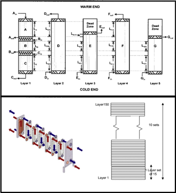
The dynamic modeling of plate and frame and spiral wound exchangers is a much more challenging task. These exchangers are mostly multistream exchangers with very close temperature approach. For plate and frame exchangers, the actual geometry and configuration becomes important in developing high fidelity models. These exchangers are characterized by a number of layers, through which the different fluids pass (Figure 4). Fins are used to increase the heat transfer area. The layer patterns can be repeating in these exchangers. The fluid volume in the various passes is determined by the geometry of the exchanger.
One way to model the plate and frame exchanger rigorously is to utilize a distributed modeling approach with discretization. This would result in partial differential equations to model the heat transfer along the exchanger length. This involves discretizing the exchanger with distributed model for mass and heat balance. One important parameter here is the heat transfer coefficients, which can be computed in a rigorous manner using empirical correlations. Normally, fixed heat transfer coefficients that are scaled with varying Reynolds numbers are used for computations. This will not capture heat transfer under conditions of phase change in the exchanger. Correlations are available for these exchanger heat transfer coefficients based on geometry. These correlations normally provide the Colburn number (Jh) as a function of operating conditions and can be obtained from the literature or the exchanger vendor. The heat transfer coefficient can then be determined using Equation 1 for Nusselt number.
where Nu is the Nusselt number, Re is the Reynolds number, Pr is the Prandtl number and Jh is the Colburn number.
The heat transfer between the fluid and the metal can then be calculated using Equation 2:
where a is the film heat transfer coefficient, A is the heat transfer area and Tmetal and Tfluid are the metal and fluid temperatures.
The overall heat exchanger can then be solved using the common wall equation, which assumes one metal at a single temperature. The equation for cell i can be given as:
where CP is the metal specific heat capacity, Timetal is the metal temperature for cell i, aij is the film heat transfer coefficient, Aii is the heat transfer area for cell i and fluid j, and Timetal and Tifluid are the metal and fluid temperatures for cell i.
For the fluid, the equation can be given as (for cell i and fluid j):
where Mij is the linear mass density, Fij is the fluid flow rate, and Hij is the specific enthalpy for the cell i and fluid j. More information about this modeling approach can be found in the discussion by Haarlemmer and Pigourier (2008).
The modeling of hydraulic phenomenon in the exchanger is another important consideration. This determines the pressure drop in the plate and frame exchanger. The pass hydraulics can be represented in detail by rigorously modeling the pressure drop along the pass. This method involves discretization along the pass length and is computationally very intensive.
The plate and frame modeling approach using discretization is computationally very demanding. This may not be practical for applications where simulation speed is important. An alternate approach is one that approximates the exchanger and splits into a few zones for modeling purposes. As a simplification, the heat transfer coefficients can be fit to match the exchanger performance. The drawback with this approach is that this may not model the heat transfer during the phase change phenomena accurately. For holdup calculations, each pass can be treated as a single holdup. Computational demands are reduced significantly with these approximations.
The dynamic modeling of spiral wound exchangers used in LNG processes is another challenging area. For these exchangers, the use of simplified models may not adequately capture the actual performance under all operating conditions. First principle model for tube bundles that employ fundamental balance equations and thermodynamic calculations is preferred. The modeling of a spiral wound exchanger with an axially distributed model for material flows and an axial with radial distributed model for heat transfer has been reported by Stephenson and Wang.
Separators
The two-phase and three-phase separation vessels are common equipment in process plants. These are modeled in high fidelity dynamic simulation with volumes, nozzle details, and elevations.
One of the important things to note for the separators is the mixing efficiency in the vessel. The default option in many commercial packages is to use perfect mixing of the incoming stream with the material already in the vessel. This may not be a valid assumption in certain cases, especially where the vapor entering the vessel does not mix with the liquid well. In these cases, mixing efficiency can be used as a parameter to adjust the extent of mixing in these vessels.
Process control
The accurate modeling of process control schemes in the LNG plant is very important in dynamic simulation. The responses of these controllers impact the overall dynamic response of the closed loop system and have to be accurately captured. This includes both the process control functionality and the control algorithms.
The base regulatory controllers are easily modeled using the proportional, integral, and derivative (PID) controller functionality. The main issue here is the type of the PID algorithm. The commercially available distributed control systems utilize different PID control algorithm equations. These may not be the same as the ones utilized in the simulation model. If the dynamic model is used for rigorous tuning, this may become a determining factor. The next level of control scheme is the advanced regulatory controls like ratio control, cascade control, and FEED-forward control. These are also modeled easily in the available simulation tools or with custom modeling equations.
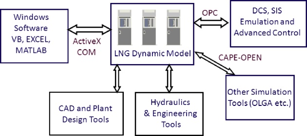
Another key consideration in LNG plant process control is the compressor antisurge control and the master performance control systems. These control systems are usually separate from the plant distributed control system (DCS). The high fidelity modeling of these systems can be important for certain applications. It is possible to replicate the functionality of these control schemes in the simulation environment. This requires replicating the various antisurge control func-tionalities and their interactions. Another option is to use an emulator for the antisurge control system, which is supplied by the vendor. These emulators can be connected to the main process model and run in parallel to capture the exact dynamics of the antisurge control system. Ethernet and Object Linking and Embedding (OLE) for Process Control (OPC) server interfaces are available to provide the data link between the emulator and the plant model. These standards can also be used to interface the dynamic model with various third-party applications as shown in Figure 5.
Fidelity and details in LNG plant dynamic models
The amount of detail and the fidelity of the dynamic models are determined by the objective of the study and the required model speed. The dynamic models can be very detailed, but this would increase computational demands and slow down the simulation, making it less useful. For applications where real-time run is required, this is not acceptable. Hence, a balance needs to be made between the level of details in the model and the simulation speed achieved.
One of the key parameters in the simulation is the integration step size. This parameter is dependent on the dynamics of the system that needs to be captured. For simulations where short time-scale events are important, very small step sizes need to be used. Compressor trip simulations are an example of this. For operator training applications, larger step sizes can be utilized as longer time scale phenomena is investigated.
Engineering studies
The dynamic simulation model used for engineering studies has to include sufficient detail for the problem under study. These models are run offline, and hence do not have to necessarily run in realtime. Still, the simulation time and the model complexity must be within reasonable limits. The size and complexity of the model depends on the scope of the study and the process units involved. A lumped parameter modeling approach is normally used for plantwide simulation for engineering studies. The hydraulics and pressure profiles are obtained from the isometric layout information for the plant, if available. This is used to calculate a lumped conductance value and volume for the various pipe elements. For applications where detailed hydraulics with momentum balance capability is required, more specialized models can be developed. Vendor-provided compressor curves are used in modeling the compressors. Actual equipment sizes are used for vessels, heat exchangers, and other equipment. Control valves are modeled with appropriate actuator dynamics, control characteristics, and valve sizes. The process control aspects of the engineering studies model include only those details that are relevant to the study. The engineering studies model is thus highly dependent on the study scope, and should be representative but is not intended to be a replica of the LNG plant.
Operator training simulators and other applications
The dynamic model used for LNG plant operator training has to run in real-time or faster to be a realistic tool for training. Hence, certain simplifications become necessary, depending on the model size and complexity. The model that is developed for engineering studies and control system studies can be leveraged as the engine for a startup and operator training tool. The scope of the model needs to be changed in this stage to suit the functionality. For realizing the maximum benefits of using dynamic simulation, a full functionality model (Virtual Plant) has to be developed that can perform startup, shutdown, and other studies. The following information is normally added to transform the engineering studies model to a virtual LNG plant.
- LNG process details. These details include the startup lines, bypass valves, emergency depressurization (EDP) valves, pressure safety valves (PSVs), and additional equipment that is needed to replicate the plant operation under startup, normal operation, and shutdown;
- Plant control systems details. The control functionality for Operator Training Simulator (OTS) has to exactly replicate the actual plant. Coding all the control functionalities within the process model is not practical. Rather, the control system emulations are used to replicate the plant control strategy. These emulations are linked to the dynamic process model using OPC for seamless data transfer;
- Plant shutdown/interlocks. The shutdown/interlock logic (SIS) of the LNG plant needs to be implemented for a realistic OTS simulator. These are implemented in separate script files or using the commercially available programmable logic controller (PLC) emulators.
The dynamic model with all the details is the heart of the OTS. The fidelity and robustness of the OTS depends on the scope and accuracy of the dynamic model. Normally, it is ensured that the model closely matches the plant data or design data before it is used for training purposes.
Applications of dynamic simulation in LNG
As described briefly earlier, dynamic simulation is used for various applications throughout the life cycle of an LNG plant. The key applications of dynamic simulation in LNG plant design and operations are described in the following sections.
LNG process design studies
One of the key applications of dynamic simulation is to identify improvements in the LNG process technology. This is not specific to any particular plant, but the LNG process design in general that is applicable to various plants that use the selected liquefaction technology. Steady state simulation is still the main tool in studying and enhancing the design of the process. Dynamic simulation can be a valuable addition in improving the process technology from the plant operability and reliability viewpoint.
LNG driver selection
The selection of appropriate drivers for the refrigeration compressors has a big impact on the overall economics and operability of the LNG plant. There are several factors that go into the selection of the appropriate drivers for the compressors. A number of them are related to the conceptual design, cost, and other related items. The areas where dynamic models can be of assistance here are those related to the operation of the LNG plant.
The first step in utilizing models for driver selection is to identify certain key metrics to quantify and evaluate the operability. These include:
- Time to start up the plant. Some drivers may require depressurization of the casing, which may add additional time;
- Ease of loading and balancing and the time requirement for the same;
- Time to recover from shutdown or time to recover from a compressor trip;
- The ease of load balancing between parallel machines. For example, singleshaft machines with limited speed ranges may have limited flexibility in load sharing between parallel machines.
Once the metrics are identified, a dynamic simulation model can be utilized to evaluate the various drivers for optimal selection.
LNG process sensitivity analysis
The operation of the LNG plant is affected by various parameters including the ambient temperature, feed gas composition, and equipment performance. The equipment design also has a big impact on the actual plant production rate. These sensitivities can be effectively analyzed using dynamic simulation to better understand and manage the risk. A good example is the effect of refrigeration compressor performance curves on the LNG production. The variations in the compressor head and its impact on the LNG plant production rate can be analyzed to obtain the sensitivity values. This information is valuable for the compressor vendor to optimize the design of the refrigeration compressor. Sensitivity of LNG plant production rate to several key operating and design parameters can also be obtained from dynamic models, as listed:
- Pressure of natural gas feed;
- Molecular weight of natural gas feed;
- Surface area of propane condenser;
- Surface area of propane subcooler;
- Gas turbine power;
- Ambient temperature.
This sensitivity information can be useful to optimize the process scheme and evaluate the trade-off between various parameters.
Another important application is the verification of the plant performance with the as-built equipment to verify if the margins that are part of the design will be useful for the owner. In this case, the simulation can be used to identify the production above the guaranteed value that can be achieved. This would validate the additional economic benefit gained from the in-built margins in the design. This information can also be valuable in evaluating the ability of the overall plant design to handle the extra throughput from the design margins. Identifying these bottlenecks would enable appropriate debottlenecking to handle the extra LNG plant feed due to the available margins.
Other process studies
Other applications of dynamic simulation in the process design area include its use to reduce the weight of offshore LNG installations. In this case, the simulation can be used for material selection and to optimize the size of equipment for an offshore environment. The material selection is impacted by the maximum pressure, maximum velocity, and forces, which are determined using simulation for startup and other transient operations. Alternatives like Fiber Reinforced Plastics (FRP) can be evaluated as an alternative to metallic pipes. In addition, this tool is valuable in reducing the overdesign of the equipment by optimizing the margins, thus saving space and weight.
Compressor antisurge system design
One of the key applications of dynamic simulation in LNG plant design is the development of an antisurge control system for the refrigeration and other compressors. The protection of compressors from surge is critical as reliable operation of these compressors is important for overall plant availability. The main objective of the antisurge control system is to prevent the compressors operating in the surge region. The operation of the machines in the surge region is damaging for the compressor impellers due to rapid flow reversals that can occur under these conditions.
There are two distinct aspects of antisurge control system development where dynamic simulation models are valuable. First is the ability of the system to maintain safe operation away from the surge region during deviations around the normal operating point. This is accomplished by the antisurge control system. The second is to prevent surge during shutdown scenarios, where the compressor rapidly coasts down to a stop. This machine protection during shutdown may be done by the safety instrumented system or by other means.
Verification of antisurge control performance under normal conditions
During normal plant operation, the process is affected by various disturbances that can move the compressor operating point toward surge. The antisurge control system will manipulate the antisurge valves to maintain the operating point to the right of the surge line. The antisurge valves need to be sized and selected to enable the operation to the right of the surge control line under these conditions. The design of this functionality is normally done by the antisurge control system vendor. Dynamic simulation is not needed to size the valve to prevent surge during normal operation. But it can still be used to provide adequate verification of the ability of the antisurge valve and the surge control al-gorithms to prevent surge under all possible scenarios.
The verification of antisurge control performance involves various operational scenarios. Some example scenarios follow. Other scenarios specific to the process under investigation can also be identified.
- Inadvertent closure of suction or discharge valves on the compressor;
- Trip of one compressor affecting the other;
- Failure of antisurge valve on one stage of a multistage compressor affecting the other stages.
These scenarios can be simulated to ensure adequacy of surge control margin, antisurge valve size, speed, and the antisurge control algorithms that are used.
The key to performing very accurate verification of antisurge system performance is having the right control algorithms in the model. In the past, the use of an actual control scheme in the model meant using the actual antisurge control hardware. Since this was a cumbersome task, most of the antisurge control schemes were emulated in the dynamic model. This could be adequate, but some fidelity is sacrificed. Recently, the soft emulators for the antisurge control system have become available, and can run in a computer. This can be connected to the dynamic model via OPC interface, whereby the process data is sent from the model to the control emulator and the valve outputs are sent back to the model. The various disturbances can be tested in this realistic environment. The same configuration files for the compressor control system that are used in the field can be used for this test. This way, the enhanced fidelity of the overall system can be used to develop reliable solutions to protect the compressors in the field.
Design of antisurge system for shutdown scenarios
The other application of dynamic simulation for antisurge control system development is the sizing of the antisurge valve to prevent surge during a machine emergency shut down (ESD). The ESD of a compressor involves the sudden stop of fuel gas to the gas turbine (or loss of motor power). This results in a loss of shaft power within a short time (typically 100 milliseconds or similar time duration). For electric motor drives, the loss of power happens even faster. The compressor will coast down depending on the inertia of the compressor-turbine string. The rate of coast-down is determined by the energy balance that relates the compressor power, inertia, and rate of change of speed as given below:
where Wdriver is the driver shaft power, Istring is the inertia of the compressor-driver string, Nstring is the speed of the string, Compression Power is the total compression power for all the compressor stages, and Losses denote the friction and windage losses in the system. For the strings where driver and compressor are at different speeds, appropriate string inertia can be calculated as:
where Idriver is the driver inertia, Icompressor is the compressor inertia, and Ndriver and Ncompressor are the speeds of driver and compressor, respectively. The string inertia in this case is with reference to the driver speed. If present, the gear and coupling inertias needs to be accounted for in a similar manner.
The antisurge valve and other system parameters need to be selected to protect the machine during coast-down from full power to a complete stop. This is especially important at high speeds, where the compression power is high and surge can be damaging to the impeller. A dynamic analysis can be performed for the compressors to ensure that the antisurge valves are sized adequately and that the stroke times of the antisurge valves are appropriate.
The input data to the dynamic simulation is very important in the simulation. The key inputs that determine the performance of this analysis are as follows.
- Compressor performance curves and the rotational inertia. The actual performance curves are required along with accurate values of rotational inertia for the string;
- Piping layout. The layout is important in determining the final size of the antisurge valves because it determines the suction and discharge volumes. Further, the hydraulic resistance is a determining factor in the overall system behavior;
- Shaft power decay. Electric motor drivers lose power instantly during trip. Gas turbine drivers have residual power even after the trip signal is initiated. This is due to the fuel gas valve actuation time and the holdup in the system that provides residual power.
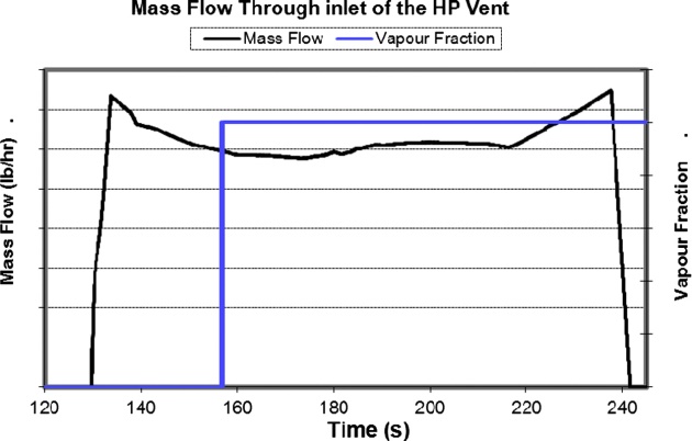
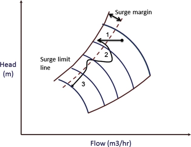
The typical desired compressor coast-down response during ESD is shown in Figure 6. Here, the compressor initially moves toward the surge line due to the valve opening time and the time for the flow to reach the suction from discharge. In the subsequent phases, the compressor moves away from surge and coasts down safely.
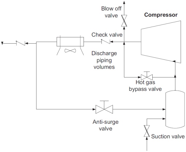
Several parameters affect the dynamic response during the trip and can be used to design the system for effective compressor protection. Some of the considerations in the design of an effective antisurge system are listed as follows (Figure 7).
- Antisurge valve sizes and valve timing. The antisurge valve size needs to be large enough to provide adequate flow for machine protection. Also, they need to open fast to prevent trip surge. Normally, 1 second or similar is utilized for the opening time;
- Suction and discharge valve timings. The compressor may have to be isolated fast to prevent the need to pressurize/depressurize the additional system volume;
- Volume of the discharge piping and suction piping. It would be beneficial to minimize the piping volumes on the compressor discharge to the valve. This is especially true for cases where the air cooler is in the loop and can be located close to the compressor discharge in the layout;
- Check valves to isolate volumes. It may be beneficial to put additional check valves to isolate and reduce the volumes;
- Hot-gas bypass for antisurge protection. For systems with discharge cooler and large volumes, a hot gas bypass option can be beneficial, as this reduces the volume in the antisurge loop;
- Blow-down valves. For certain systems, blow-down valves can be used to reduce the discharge pressure right after trip. This is normally not a preferred option.
These various options can be analyzed using dynamic simulation to determine the effectiveness of a potential solution. In some cases, a combination of options may be required. Dynamic simulation is valuable in determining the most cost effective and robust solution for antisurge protection.
The application of dynamic simulation for designing the antisurge system for refrigeration com-pressors in an LNG plant is well documented in the literature. This includes the refrigeration compressors in the Cascade Refrigeration LNG Process and the MR and other compressors in the APCI C3MR process.
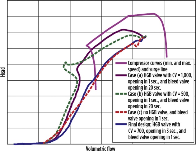
There are cases where antisurge valves sized for ESD may not be sufficient to provide surge protection during startup. In the example reported, the startup of the compressor with propane needed a control valve size (Cv) of 2 600 (as opposed to 1 600 required for ESD surge protection). Further, the startup with N2 or defrost gas needed a Cv of 3 000. In this case, it was necessary to make the startup Cv a function of the case considered by clamping the valve size appropriately. In addition, the various options in the design of the antisurge system for the MR compressor were studied here. This included using the bleed valve, hot gas bypass valve, and discharge valve to flare to optimize the design (Figure 8).
Other applications in compressor systems
There are other applications of dynamic simulation in the design and operation of compressor systems. One of them is for evaluating the effect of deviations in compressor curves between two parallel refrigeration compressors. This difference will have an impact on the load balancing between the two strings, especially for single-shaft machines with limited speed ranges. In this case, suction throttling valves may need to be used for load balancing. The impact of these deviations on the compressor operation can be tested prior to operation. In one case, it was found that a 5 % deviation can cause one of the compressors to operate in recycle, thus reducing the overall efficiency.
Other applications of dynamic simulation in compressor systems include developing startup pro-cedures, developing compressor control strategies, and tuning the various control loops. The application of simulation in developing control strategy for an MR compressor was reported by Patel et al. (2007). In this case, the low pressure (LP) and medium pressure (MP) compressors, which are in the same string, experienced surge when the high pressure (HP) MR compressor in a different string was shut down. The normal surge detection and control was not sufficient in this case due to the delays in the valve stroke and actuator response. Feed-forward control actions that manipulate the antisurge valves for LP and MP compressors upon trip of the HP stage were developed to prevent surge in this application.
Operability and controllability analysis
Dynamic simulation is a valuable tool in evaluating the design and operability of the LNG plants in the early engineering stage. This helps to mitigate any risks related to operability during plant startup and operation. Further, the simulation can help to optimize the design by reducing any unnecessary margin. The operability of the entire plant is determined by both process design and the control system design. The changes in control schemes are easier to make at later stages. On the other hand, process design changes in later project stages are much costlier. Simulations can be carried out in the early design stages, where the changes in the design are identified and made with minimal adverse impact on the project cost. This eliminates any costly rework in the field after startup and commissioning.
The dynamic simulation-based operability analysis for the LNG plant can be of different scope, as follows.
- Equipment level. At this level, the individual equipment operation is analyzed. This could be the operation of gas turbines, expanders, etc. The main benefit is to verify how the individual equipment fits into the overall plant operation;
- Unit level operability. In this case, the operation of an individual unit is analyzed. This could be an amine system, fuel gas system, boil-off gas system, or steam system in the plant. The main concern here are the interactions within the unit and the impact on the unit controllability;
- Plantwide operability. In this case, the operation of the entire plant is analyzed to identify any areas of concern. This could be startup, shutdown, or other plantwide operational scenarios.
There are several examples of operability enhancements that have been accomplished for LNG plants using dynamic simulation. Some of these are listed here:
- One of the main concerns in LNG plant is smooth plant startup. The value of simulation analysis here is discussed separately in the next section;
- Another important issue related to LNG plant operability is the ability of parallel refrigeration compressor systems to operate reliably when one of the compressors trips. This has been studied for both APCI C3MR and cascade refrigeration processes. The main area of concern here is the possibility of overloading and tripping the parallel compressor train, when one of the compressor strings trips. Suitable control strategies to prevent this overload trip of parallel turbine were developed using dynamic simulation. In addition, trip of helper motors, wherever used, can be analyzed for any risk to the overall operation;
- For APCI C3MR plants, the failure of Main Cryogenic Heat Exchanger (MCHE) is also an important issue. The effect of this on the overall plant reliability is realistically analyzed using dynamic simulation;
- For systems where the electrical system performance can have an impact, the model can be updated to include the performance of the electrical system. In this case, the effect of electrical faults or trip of Load Commutated Inverter can be analyzed using a suitable dynamic simulation model;
- The operability of fuel gas systems to ensure appropriate fuel gas header pressure and fuel properties during transients;
- Application of surge analysis for the LNG loading line. This involves analyzing the pressure surge in the loading line under various scenarios like valve closure. This can be used to identify and implement surge dampening devices in the system;
- The confirmation of operability of NGL recovery unit in the LNG plant as reported by Masuda et al. (2012). In this case, dynamic simulation was used to verify the operability and controllability during startup and shutdown of the expander, turndown of the NGL recovery unit, failure of ASV valves in the residue gas compressor, and the trip of the residue gas compressor.
These are some examples of improvements in operability achieved using dynamic simulation. Other similar concerns related to LNG plant operability and controllability can be addressed using simulation.
LNG plant startup simulations
One of the key benefits of dynamic simulation is the ability to test startup of the LNG plant before field commissioning. Startup is inherently dynamic and the use of steady state process models is not appropriate for this exercise. This is even more important for the plants where design changes are introduced. This inherently brings in additional risks as to the ability for a smooth plant startup. Some of these risks can be addressed early in the design stage using dynamic simulation. The important aspects of the startup applications are detailed in the following.
Startup procedure development
One of the startup applications of dynamic simulation is the development of a startup procedure for the plant. This is very relevant in the case of LNG plants with design modifications, which may introduce issues with startup procedures. Identifying these issues early in the design can help to modify the design to handle issues. This also helps to automate certain startup steps in the DCS, which can help reduce the variability in the startup with different plant operators.
Another very important benefit is having a well-defined startup procedure ready for the field startup. This procedure can further be refined in the field. The key to startup of the LNG plant is the liquefaction section, especially the refrigeration compressor systems. These can be verified and refined with dynamic simulation.
An example of the use of dynamic simulation for startup enhancement is its use as a tool to tailor the cooldown procedure for the loading line and hence minimize the use of cold gas and LNG. Another example of enhancing startup using simulation is the solution to the issue of loading and balancing of two parallel trains. The development of a procedure to do this using dynamic simulation is reported for APCI C3MR plants and cascade processes; Valappil et al., 2011). For the C3MR process, the suction drum for the machine in recycle needs to be precooled by an appropriate gas stream. The rate of cooldown is controlled by the antisurge valves. Once the temperatures are equilibrated, the block valves can be opened and the forward flow through the check valves can be established.
Verification of driver capability and startup conditions
The refrigeration compressors and the drivers are some of the key equipment in the LNG plant. These machines have to be started up without any operational issues. The drivers for these compressors could be gas turbines, steam turbines, or electric motors. It needs to be ensured that these drivers have enough power to bring the entire compressor string from a shutdown condition to normal operating speed. This could be an issue for single-shaft gas turbine and electric motors, which have limited torque available during startup at speeds lower than the normal operating speed. Dynamic simulation can be utilized to verify the driver torque adequacy during startup.
A related issue is the startup conditions that are used in the compressor loop. The initial pressure used for the startup has a big impact on the torque requirements during the ramp-up to normal speed. Hence, the selection of right starting pressure is critical, if it needs to be different from the settle-out pressure. These starting conditions can be fine-tuned and selected using simulation. A related concern is the process conditions in the compressor loop during startup. The possibility of encountering vacuum conditions in the compressor suction can be verified for startup using low pressures. This information is valuable to ensure the right design pressures are used for the piping and equipment that can experience low pressure conditions. It may also be required to ensure that the antisurge valve openings are clamped during the startup to prevent excessive flow through the stages. The suitable valve openings can be developed using simulation analysis.
The key input here is the driver speed-torque curve that defines the capability of the machine at various speeds. The torque available has to be sufficient to provide both the compression power and the acceleration power. A certain amount of margin also needs to be provided (Figure 9). The gas turbine has a predetermined speed acceleration rate that can be programmed into the model for simulation of startup.
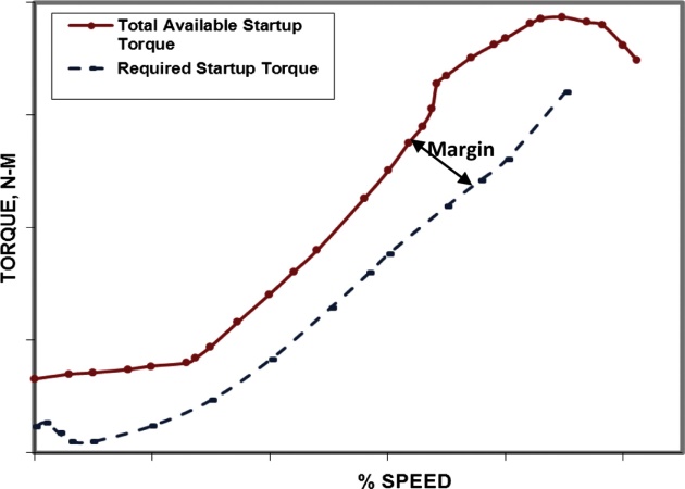
The model would then calculate the total torque based on the operating point on compressor curves and the rotational inertia of the string. Another important factor that should be included here is the possible seal gas leakage. This can add to the torque requirements during startup as mass is added to the compressor loop, resulting in higher torque demand.
Dynamic optimization of LNG plant design
The optimization of the plant design is normally carried out using steady state models, as these models are capable of evaluating multiple designs seamlessly. This is important for optimization with a large number of variables. There are benefits to be gained from using dynamic models for other optimization purposes during the design phase of the LNG projects. There are costs associated with equipment parameters like surge volumes, control valve sizes, and so on, which are provided to satisfy certain dynamic performance needs. These costs are determined by dynamic characteristics of the system. The ability to optimize these parameters using simulation and optimization tools is valuable for improving the profitability of LNG plant design.
One area of application of dynamic optimization are the offshore LNG plants, where the weight or size of equipment can be a constraint. Dynamic optimization is a valuable tool for reducing the weight by optimizing the size or selecting a different material. Another example is optimizing the size of propane condenser in the APCI C3MR process using simulation.
Dynamic optimization is best performed by utilizing an optimizer linked to the dynamic simulation model. The economic parameters for the optimization have to be input along with any other constraints. These could be limits on the process variables or constraints on optimization parameters. The optimization tool is utilized to determine the best design, maximizing an objective function (alter-natively, minimizing cost). For this, repeated simulation is needed and the performance of each run collected and analyzed. The adjustable parameters like antisurge valve sizes can be varied to determine the optimum point and determine the exact benefits from reducing the capital cost of the plant via optimization.
Another important area of application is determining the maximum plant capacity and the best operating variables to optimize the plant production. This is closely related to debottleneck and advanced control applications. The example reported by Ismail et al. (2004) opti-mizes the LNG production by varying key operating parameters like Inlet Guide Vane (IGV) angle of a LP MR compressor, Inlet pressure of a LP MR compressor, Outlet pressure of a MR expander and the MR composition. The optimization is done with the constraints on refrigeration driver power, outlet pressure of a heavy MR expander, IGV angle and the temperature approaches in MCHE. For the cascade refrigeration process, similar optimization can be accomplished by varying refrigeration compressor suction pressures, condensing pressure, and other load balancing (between the three refrigeration systems) handles in the process.
Relief system design and safety scenarios
A properly designed relief system is very important for the safe and reliable operation of the LNG plant (refer to Appendix 3). Hence, the proper sizing of the relief valves is a key part of the engineering design of the plant. The majority of the relief valves are adequately sized using the traditional calculation methods. There are certain scenarios like a compressor blocked outlet or general power failure that are better analyzed through dynamic simulation. In these cases, various competing and time-dependent events can become active, which can impact the relief flow rates. Also, dynamic simulation accounts for the actual volume and inventory of the refrigeration systems in the LNG process. This helps to provide more realistic relief rates during various transient scenarios.
One of the LNG process relief cases where dynamic simulation has found applicability is the compressor blocked outlet case. The use of dynamic simulation in analyzing the inadvertent closure of the compressor discharge block valve and the propane receiver outlet block valve for APCI C3MR process has been reported. This was utilized to verify the adequacy of the relief and flare system and the size of the bypass around the relief valve. During a blocked outlet scenario, different scenarios can happen, including the compressor going into recycle and the chiller pressures continuing to rise. Further, this can result in overloading of the turbine driver and bogdown, resulting in turbine trip at minimum speed. The bogdown of the gas turbine and its impact on the possibility of relief rate reduction were analyzed.
Another application is the scenario of General Power Failure (GPF) and the determination of relief flow rates during this event. Several independent events are triggered by a GPF, the cumulative effect of which is well analyzed by dynamic simulation.
A related application of dynamic simulation is the analysis of flare system adequacy to handle various relief scenarios. Simulation can also look at the actual timing of various relief scenarios and the ways to mitigate the maximum relief flows, hence preventing the overdesign of flare systems. An example of this is the relief due to loss of power for the propane compressor air-cooled exchanger fans in the APCI C3MR LNG process. Providing emergency power to some of the air-cooler fans was identified as a more cost effective alternative to increasing the flare header size in this case.
Dynamic simulation is also being used as a tool for designing the flare system itself. Here, the dynamic model of the flare network is developed with the actual piping and equipment data. This is used along with the various relief or emergency depressurizing scenarios to identify the conditions in the flare header and knockout drums during the flare event. These conditions are realistic estimates and can be used to optimize the design of the flare system.
Another area of application of dynamic simulation is the analysis of safety scenarios and HAZOP scenarios. These are scenarios where the plant could potentially reach an unsafe operating condition. The possibility of attaining such conditions can be evaluated to ensure that the proper preventive measures are built into the design.
Plant troubleshooting and operational support
A very key benefit of developing a high fidelity LNG plant dynamic model is its use in assisting plant operations. The model can be validated with plant data at frequent intervals to make it an adequately accurate representation of the LNG plant and used for “what-if” or other operational studies.
The main application of a validated plantwide dynamic model is plant troubleshooting, where the model is used to identify the root cause for certain plant events. These troubleshooting studies involve first replicating the plant scenario in the validated model. Then, the dynamic model is used to identify potential options for mitigation. A number of operational problems can be investigated and mitigated with this approach.
Another very important value of having an LNG dynamic model is providing operational support. This involves providing the right operating setpoints under various plant conditions like ambient temperature, feed compositions, and so on. The dynamic model that is representative of the plant can also be used to identify better operating strategies for the LNG plant.
Plant production enhancements and debottlenecking
There is a significant emphasis on utilizing the existing natural gas assets to their maximum potential. The first step in achieving this is operating the existing LNG plants at their maximum capacity. Beyond that, there are economic incentives in debottlenecking the existing LNG plants to increase their capacity or availability. There are various options available to perform the debottlenecking of existing plants. The evaluation and selection of the best options to increase the plant capacity is important for optimum return on the investment. An overall plantwide dynamic simulation model is a useful tool to perform the evaluation and optimization of the various debottlenecking options.
The main objective is to identify and remove the capacity limiting constraints in the plant. Once the existing constraints are identified, various options are considered to debottleneck the LNG plant and are studied with the simulation models. There are various options to perform the debottlenecking of existing plants. These include:
- Upgrades or modifications to existing equipment;
- Replacement of existing equipment with ones that provide higher capacity;
- Changes in process configuration or conversion to alternate technologies.
The dynamic model can be used as a tool to screen the various debottleneck options and to identify the most economical one before the detailed engineering design. The dynamic model is an actual replica of the existing plant, and can be used for rapid screening of multiple debottleneck options. This is especially valuable when evaluating various combinations of options.
The simulation model needs to be first validated and baselined with the operating data from the LNG plant. This is essential to establish a valid baseline for further debottleneck simulations. The simulation models may be built during the engineering and construction phase of the plant to evaluate and predict the plant performance prior to the initial operation. This initial model needs to be updated to incorporate actual tested equipment performance data and baselined to reflect the actual plant behavior. The model parameters are tuned with the actual plant data that is reflective of the normal plant operation over time. The main focus of the baselining exercise was to validate the performance of the refrigeration systems (especially the compressors and gas turbines) and other constraints against the plant operation.
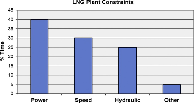
It is important to identify the existing plant constraints before performing any debottleneck evaluations. These constraints vary with the operating conditions like ambient temperature, feed composition, and so on. Some of the main constraints that limit production in LNG plants are related to the refrigeration compressor drivers. Also, various other equipment limitations and hydraulic constraints may be present in the plant. In addition to steady state models, a plantwide dynamic model provides a suitable tool to identify these existing plant constraints over the range of operating conditions. The percentage of time annually that each constraint is active can be determined from simulation to identify the debottleneck options to be selected (Figure 10).
Once the existing constraints are identified, various options to debottleneck the LNG plant can be studied. Of particular interest are plant changes that can be made with minimum downtime or within the downtime required for other purposes. For example, gas turbine drivers can be upgraded to those with higher power ratings.
The simulation models can be run with the actual field conditions to identify the plant performance with these debottleneck modifications individually or in selected combinations. The incremental LNG production is estimated at various times of the year to obtain an annualized production increase (Figure 11).
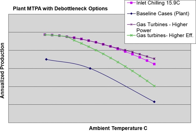
This is important to optimize the selection of LNG plant debottleneck modifications that can be used in estimating the return on capital investment.
Control system checkout
The dynamic simulation model can be used for a variety of control system related applications. One of the potential applications is the determination of the right control structure in the early stages of the project. Systematic ways of analyzing the process controllability using the dynamic model are available at present. This helps to establish the economic trade-off between steady state design and process controllability. These studies would have to be done in the early stages of the project, preferably in the FEED stage. Since these decisions are more qualitative in nature, the lack of detailed equipment information should not be a serious limiting factor in these applications.
The other important use of dynamic simulation is the selection of appropriate tuning parameters for the plant. Usually, the tuning parameters from a similar, previously constructed plant are used or the control loops are tuned on-site during the commissioning phase of the project. This prolongs the startup-commissioning time, thus making it economically very inefficient. The availability of a dy-namic simulation model makes it possible to tune the control loops off-line in advance using established tuning procedures. These can then be fine-tuned quickly on-site during the commissioning. These studies can be performed during the EPC stage or precommissioning.
The other major application of dynamic simulation in control system studies is in the checkout of the plant control system prior to commissioning. In traditional practice, simple tie-back models are used for this purpose. This helps to confirm the input/output (I/O) integrity, but does not assist in other studies and does not include any process knowledge. A high fidelity dynamic simulation model provides an alternative to check the control system connections, the control logic, and the tuning parameters before the commissioning phase. This also helps to provide the framework for a future operator training simulator development. The LNG plant commissioning time saved by better checkout and operator training adds economic value to the project.
The process control system landscape has changed with the introduction of the digital fieldbus, as explained in Chapter 6. This has added further capability in performing model-driven control system checkout in a transparent manner. High fidelity dynamic simulation models can be linked to the emulation of the control system to perform the checkout in a single PC. Linking between the dynamic simulation models and control system emulations can be effectively performed using standards like OPC and CORBA (Figure 5). This avoids the need to purchase the control system hardware to do the checkout and operator training. Also, the hardware independence of the emulation tools makes it ideal for a system-independent approach.
Operator training simulator
A high fidelity plantwide LNG dynamic model can be integrated with the control system emulations for use as an operator training simulator (OTS). An OTS based on such a model is a true replica of the plant, reflecting both the process and control elements. Control system emulators are useful to replicate the exact plant control strategy (most commercial DCS systems have an emulator that can be used for this purpose). The shutdown/interlock logic (SIS) of the plant is also implemented in the OTS. This logic is either implemented in separate script files or by using commercially available programmable logic control emulators. The OTS also utilizes the actual operator displays to capture the exact control room environment. The field operator station is replicated to enable the field operated valves, hand switches, and other functionalities. The instructor station is used to start and manage the training scenarios and perform operator evaluations as shown in Figure 12.
The benefits of using an OTS in LNG plants are several, including:
- Many of the LNG plants are located in remote areas, where experienced operators are not readily available. Hence, training the operator on an OTS is valuable in improving the plant availability and reliability. This training enables the operators to learn the functionality of the plant automation system and operating procedures in an offline environment;
- The OTS allows for complete control system checkout prior to plant commissioning. This enables engineers to resolve any issues regarding graphics or control logic coding early in the project;
- Operating personnel can also use the OTS for training purposes to ensure a smooth plant startup and commissioning. Feedback from operating personnel on the OTS also helps to provide the framework for the future OTS development;
- The OTS can be used for operational support once the LNG plant is up and running. This includes design changes, debottleneck analysis, troubleshooting, etc.
The training scenarios performed in an OTS include startups, normal operations, and abnormal situations. This abnormal situation training is very valuable, as these events occur rarely and the operators are not exposed to this in the plant.

The selection of these malfunctions to train the LNG plant operator is the key to realizing maximum benefits from training. Some of the typical malfunctions that are simulated in an LNG plant OTS are:
- Ambient temperature changes;
- Failure of air cooler;
- Failure of the amine pump;
- Foaming in the amine column;
- Trip of refrigeration compressors;
- Trip of Main Cryogenic Heat Exchanger;
- LNG transfer pump failure;
- Trip of boil-off gas compressor.
The relative performance of the operator in handling these malfunctions can be tracked using a Trainee Performance Monitoring (TPM) tool. This can be set up by the instructor using certain critical parameters and their limits that should be honored. This way, the operator can be trained to effectively handle these abnormal situations in addition to the normal operation of the plant.
To realize the benefits of OTS fully, the training simulator should be developed during the engi-neering and construction stage of the project. The OTS ideally should be in the field anywhere from 6 months to a year before the startup. This way, the operators can be adequately trained and prepared for the plant startup and operation.
A novel approach to development of an OTS system for a Yemen LNG plant was described by Rabeau et al. (2010). A dynamic simulation model was used extensively in this case for the engineering design of the LNG plant. The same model was then used for development of OTS. Different phases of OTS development were used with a different OTS in this case, as shown:
- Dynamic Engineering Simulator. Simulation model used for engineering studies that does not include any DCS emulation or consoles;
- Early Operator Training Simulator. This is a simplified emulated OTS system with Human Machine Interface (HMI) that is used for process courses;
- Extended Early Operator Training Simulator (EEOTS). This is a more detailed OTS with emulated controls and DCS HMI;
- Operator Training Simulator. Full OTS with DCS and ESD stimulation and actual DCS consoles.
The Emulated OTS was used in this case for several process studies. The EEOTS was used for developing startup procedures. Since this was available several months before the actual plant startup, EEOTS was also used to train operators extensively before startup.
Advanced process control development
APC/optimization has established itself as a widely used technology in the process and other industries, including LNG plants. The implementation of APC/optimization is currently done after the plant has been operational for some time. Even in the grassroot plants, this is the normally accepted practice. There are some drawbacks to this implementation philosophy though. Recently, dynamic simulation is being used for developing APC applications before field implementation in LNG plants. This helps to minimize the impact on the plant operation during APC implementation.
The dynamic models developed for various LNG project stages can be used for various APC applications (Figure 13). In the front-end stage, it can be utilized for design studies. The EPC stage dynamic model can be used to validate the regulatory control systems and to prototype the advanced controller.
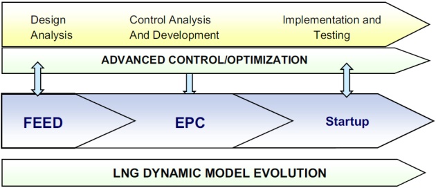
The dynamic model that is validated with plant data is a valuable asset in optimization and advanced control studies. This model can be used for estimating the potential benefits of advanced control, performing plant tests to obtain preliminary models, and testing the APC/optimization under various operational scenarios.
- Analyzing LNG process design for APC. The analysis of process design in the early plant life cycle stages can verify the operability of the plant at optimal conditions after plant startup. This involves ensuring that the right operating constraints are considered and that no auxiliary variable becomes a limiting factor in optimization. Dynamic simulation can be used in the early project stage to identify the plant operating envelope after the plant startup. From a design point of view, it is important to consider the undesirable constraints that can become active during the operation. These can be identified during the operating envelope runs. This way, it can be ensured that the advanced control can operate the plant at proper constraints during the future plant operation;
- Designing regulatory control systems. The regulatory control layer of a typical plant is designed and finalized during the detailed engineering and construction phase. The instrumentation and control system design that is done during this stage is intended for normal plant operation. The implementation of advanced control requires additional instrumentation or changes in the regulatory control layer. Identifying these changes or additional control features in the engineering phase will prepare the plant for future advanced control implementation;
- Estimating benefits from LNG plant APC. A dynamic model that is validated with plant data can be used for estimating the potential benefits of advanced control, performing plant tests to obtain preliminary models, and testing the optimization under various operational scenarios. It is important to accurately estimate the benefits from optimization to justify its implementation. In most cases, purely plant data driven methods have been used to estimate the APC benefits. A different way to estimate the benefits is to actually simulate the operation of the plant with optimization and then compare it with a baseline operation;
- Evaluating plant performance with APC. The performance of the plant with optimization under various conditions can be studied with dynamic simulation. There are several advantages to doing this. One advantage is the fact that the constraints that the plant will operate normally are easily identified. Also, any changes in constraints with changing ambient or other variables can be detected using dynamic simulation. The plant operators can be trained to manage these changes.
Dynamic simulation of LNG import terminals
Dynamic simulation has found a range of applications in LNG import terminals, including safety studies, operational optimization, and rigorous hydraulic analyses. A brief description of the modeling of LNG import terminals and the various applications are given in the following sections.
Dynamic modeling of LNG import terminals
The methodology for the development of LNG import terminal dynamic models is similar to the LNG plants, as many of the unit operations are similar in nature. The main components of the import ter-minal dynamic model are the LNG storage tanks, BOG compressors, and LNG vaporizers.
The modeling methodology used for an LNG storage tank depends on the scope of the model and application that the model is used for. For process studies, where the interest is in the BOG generation and the tank level, the tanks can be modeled with the standard unit operation models. These consider the tank volume as a simple holdup at the same conditions in the entire tank. Assuming perfect equilibrium in the tank is not very accurate, and reasonable tank efficiency has to be specified. The heat leak into the tank can be calculated externally and specified or calculated based on the heat transfer parameters in the tank. The accurate heat loss calculation is important, as it determines the generation of boil-off gas. In addition, the heat gained from pumps would also contribute to the vapor generation. For more detailed calculations of the tank including scenarios like roll-over behavior, more rigorous models are needed. This is especially valuable to study the behavior of mixing of two different density fluids like roll-over. The tank model in this case needs to take into account the spatial distribution of fluid properties. This results in partial differential equations, with an accompanying turbulence model that can be solved using Computational Fluid Dynamics (CFD) tools.
The other important component of the LNG import terminal model are the vaporizers used to convert LNG to vapor. These vaporizers need to be modeled with adequate fidelity to handle the scenarios studied. Simple heat exchanger models, with parameters chosen to reflect the actual vaporizer, would be sufficient to study the operability of the system. For further exact modeling of the vaporizers, more rigorous heat transfer correlations can be used. This is especially valuable for modeling the ambient air vaporizers, used in some of the LNG vaporization processes.
Applications of dynamic simulation in LNG import terminals
Design and testing of safety and operational scenarios in LNG Terminals
One of the valuable applications of dynamic simulation is in performing safety analysis, particularly designing and testing the Emergency Shutdown systems for the LNG terminal. The design of an ESD system for the LNG terminal is critical to ensure safety. The various safety hazards can be simulated to ensure that the ESD system design is adequate to deal with these situations. If needed, the system can be redesigned or fitted with ancillary equipment. Plant personnel can define more effective safety action plans and shutdown strategies.
In addition, other operational applications were reported by Contreras and Ferrer (2005). These include the following:
- Startup and shutdown of pumps. This involves studying the transients involved in shutdown and startup of various pumps in the regasification terminal;
- Vaporizer shutdown scenario. The shutdown of LNG vaporizers is a severe upset in the LNG import terminal operations. The effect of this upset and the ability of the system to accommodate this upset can be studied;
- Failure in the BOG compressor. The failure of one of the BOG compressors during ship unloading and the resulting pressure transients are studied here.
Determining optimal operational strategy and LNG terminal responses
The optimization of LNG terminals using a dynamic model was discussed by Lee et al. (2012), whereby various operational strategies were developed to minimize the total operating cost. This indirectly amounts to reducing the generation of boil-off gas in the system. The main emphasis is to evaluate the effect of bypass flow rate and recirculation flow rate on the various terminal characteristics to enhance the operating efficiency.
The other application of simulation is in optimizing the operation of boil-off gas compressors in the LNG regasification plant. This includes determining the operating points for the various compressors to minimize the overall energy consumption. An application of this using steady state plant models was discussed in Shin et al. (2007). This can be extended to use a dynamic model instead of steady state model.
The use of dynamic simulation in studying various operational scenarios and validating control systems for the Freeport LNG terminal was discussed by Nanda et al. (2010). The main concern here was the transition from summer to winter mode of operation and its effect on the heating tower. This transition involved a change of about 30 °F for the most conservative case. A dynamic model for the entire facility was built and used to verify the plant operation during the transition. The results of the analysis were used to determine setpoints for the various control loops and to pretune the loops before commissioning. The model was also used to optimize the energy consumption by changing the setpoint of the main controllers.
Transient flow analysis in LNG flowlines
The safe and reliable operation of the LNG regasification plant is a key objective of the overall facility design. There will be a need to isolate the inventory in the system during emergency scenarios. Emergency shutdown valves are provided at various points in the process to accomplish this objective. The closing times of these valves need to be selected to ensure quick protection without adverse hydraulic transients like water hammer. The water hammer phenomena can be caused by startup or shutdown of pumps or by sudden closure of valves.
The first area of application of this analysis is the carrier unloading system, which includes the pipeline from the jetty to the LNG terminal. The closure of valves in this area can cause pressure peaks, the magnitude of which can be studied. The second area is the LNG flow from the tanks to the va-porizers, from the submerged pumps. The effect of valve closure in this area can also be evaluated. The other scenarios that can be examined include the high pressure sendout pump valve closure and LNG storage system valve closures.
Evaluating tank filling operations
The other application of simulation is to ensure that there are no rollover phenomena during tank filling operations. This can happen when LNG is added to a storage tank with LNG of different density, resulting in stratification and a sudden release of a large amount of boil-off gas. A model used to study this needs to have spatial details, which results in partial differential equations (continuity, momentum, and energy balance equations for the tank). Commercially available CFD codes can be used to solve this problem.
Case study: LNG import terminal dynamic simulation
A dynamic model was developed to study the transient performance of LNG terminals with Ambient Air Vaporizers (AAV). This model (shown in Figure 14) was used in calculating the physical properties and relieving performance of LNG at blocked in conditions.
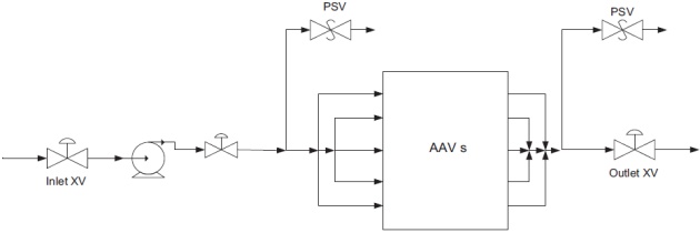
The model was also used to calculate the mass flow through the dump valve in order to prevent the system from overpressuring.
The specific objectives of the dynamic modeling exercise were as follows.
- Calculate the physical properties of relief valve discharge for abnormal heat input case;
- Calculate the physical properties of relief valve discharge for fire case;
- Estimate the withdrawal rate through the dump valve so that the system does not reach 95 % of the design set pressure;
- Estimate the settle out pressure and mass of LNG remaining in the system when the system exit isolation valve is closed after 60 seconds of the inlet valve closing.
A dynamic model for the system was constructed with AAVs modeled using heat exchanger unit operation. The pumps and the isolation valves were also included in the dynamic simulation model (Figure 14).
Simulation runs
This section presents details of different cases studied using the dynamic model.
Blocked in condition with abnormal heat input
In this case, the inlet isolation valve (XV) and exit XV of the system are assumed to close in 3 seconds. During this period the flow from the pump decays to zero. As a result of the closing of the XVs, the system becomes isolated and heat transfer occurs from the ambient air to the AAVs. This transfer of energy leads to an increase in temperature of the fluid trapped inside the system and hence results in rapid pressure rise. When the set pressure is reached the relief valve opens and releases gas to the atmosphere. The pressure response at the inlet of the relief valve was determined from this simulation.
Blocked-in condition with fire
This case is similar to the previous one. In this case, a plant fire near one of the AAVs leads to an increased heat input to the system. For the sake of simplicity this radiant heat input is assumed to be constant and limited to the bottom quarter of the length of the tubes that faces the fire. The extra heat input causes the pressure of the system to increase more rapidly. The maximum flow rate of gas when the relief valve opens is more than that for Case 1.
Delayed dumping of LNG before exit XV closing
In this simulation, the possibility of preventing overpressuring of the system by removing fluid through a dump valve is investigated. The dump opens as soon as the inlet XV is closed and remains open until the closing of the exit XV in 60 seconds. The valve Cv is varied such that the final pressure of the system after closing the exit XV does not exceed 95 % of the design pressure. The maximum flow rate through the dump valve is determined form this simulation. Plots of temperature, pressure, and fluid vapor fraction across the dump valve is given in Figure 15.

Delayed closing of exit XV
In this scenario the dump valve does not open. It is assumed that the inlet LNG valve shuts off in an ESD event, which stops the LNG flow. The AAV system outlet valve stays open for 60 seconds from the start of the event before closing. During this time the LNG in AAV gets heated. This causes the fluid to expand and flow out of the system as the downstream pressure is constant. After the exit is blocked the system pressure rises. The mass of LNG left in the system after isolation is calculated.
Opening of HP vent for depressurizing
This scenario is similar to the previous case. An HP vent is located at the exit to the AAV arrays. The exit XV closes after 1 minute of the closing of the inlet XV. After this, the pressure in the system rises as the fluid inside gets heated. When the pressure reaches a set pressure, the HP vent discharges gas to the BOG header, which is at a very low pressure. The HP vent closes as soon as the system pressure goes below a predetermined pressure. In this simulation the maximum flow rate through the HP vent was determined. Plots of temperature, pressure, and fluid vapor fraction across the dump valve are given in Figure 16.