The success of the design and operation of separation processes in the oil and gas industry at low temperatures is critically dependent upon accurate descriptions of the complex phase behavior and thermodynamic properties of the multicomponent hydrocarbon mixtures with inorganic gases concerned. For many years vapor-liquid equilibria problems in natural gas systems have been successfully solved. Yet, at present, interest has shifted to systems containing not only species in the simple paraffinic homologous series, but also to water \( (H_2O) \), carbon dioxide \( (CO_2) \), hydrogen sulfide \( (H_2S) \), hydrogen \( (H_2) \), nitrogen \( (N_2) \), to mention a few, in which multiphase phenomena can occur. For example, the situation of interest in natural gas processing is often a methane-rich stream in which the presence of a second solvent might alter dramatically the pattern of the phase behavior of the customarily liquid-vapor mixture and cause problems.
- Introduction
- Thermodynamics and topography of the phase behavior of LNG systems
- Numerical procedures for calculating the multiphase equilibrium
- Computational technique 1
- Computational technique 2
- Calculation of critical points at constant composition
- Criticality conditions
- Solution procedure
- Calculation of K- and LCST-points at constant temperature
- Calculation of phase envelopes
- Thermodynamic models
- The SRK equation of state
- The PC-SAFT equation of state
- Examples of application
- The nitrogen + ethane system
- The nitrogen + propane system
- The nitrogen + methane + ethane system
- The nitrogen + methane + propane system
- The nitrogen + methane + n-butane system
- The nitrogen + methane + ethane + propane system
- The nitrogen + methane + ethane + propane + n-butane system
Introduction
In this aspect, a neglected field of LNG equilibria work has been that portion devoted to vapor-liquid-liquid behavior. Process inefficiencies are often a result of this multiphase behavior, because the additional phase can cause unexpected separation problems.
In the cryogenic processing of natural gas mixtures, species such as \( CO_2 \) and the heavier hydro-carbons can form solids. The latter might coat heat exchangers and foul expansion devices, leading to process shutdown and/or costly repairs.
Thus, knowledge of the precipitation conditions for gas streams is essential in minimizing downtime for cleanup and repairs. However, the appearance of a solid phase in a process is not always a liability. Off-gas (primary nitrogen) either from power plants with light water reactors or from fuel processing plants can contain radioactive isotopes of krypton and xenon, which can be removed by solid precipitation. The phenomenological aspects of LLV/solid-liquid-vapor (SLV) behavior are hence also interesting because there is a need for a better understanding of the physical nature of the thermodynamic phase space.
The aim of this appendix is to reveal, examine, and analyze the challenges and difficulties encountered when modeling the complex phase behavior of LNG systems, and to compare the capabilities of two numerical techniques advocated for phase behavior predictions and calculations of complex multicomponent systems.
The appendix is organized as follows. First, the thermodynamics and topography of the phase behavior of LNG systems are briefly presented. Then, two computational techniques to predict and model complex phase behavior of nonideal mixtures and their application to LNG systems are described, followed by presentation of a numerical procedure for calculating critical points of multicomponent mixtures at constant composition. Localization of a mixture critical point is critical for the correct construction of its phase envelope. The next section of the appendix is devoted to the description of a modified new method to directly calculate critical end points (K-and L-points). Next, two representatives of the equations of state (EoSs) type thermodynamic models, which are usually the primary choice when modeling LNG systems, namely SRK EoS and PC-SAFT EoS are briefly outlined. Examples of application and discussion of the phase behavior modeling for selected binary, ternary, and multicomponent systems of particular interest to the natural gas industry are presented.
Thermodynamics and topography of the phase behavior of LNG systems
Though only a limited number of immiscible binary systems (methane-n-hexane, methane-n-heptane, to name the most prominent ones) are relevant to natural gas processing, LLV behavior can and does occur under certain conditions in ternary and higher LNG systems even when none of the constituent binaries themselves exhibit such behavior. It is also known that the addition of nitrogen to miscible LNG systems can induce immiscibility, and this necessarily affects the process design for these systems.
The qualitative classification of natural gas systems and the topography of the multiphase equi-librium behavior of the systems in the thermodynamic phase space and the nature of the phase boundaries will be addressed in this section.
Kohn and Luks (1976, 1977, 1978), who carried out extensive experimental studies on the solubility of hydrocarbons in LNG and NGL (natural gas liquids) mixtures, qualitatively classify natural gas systems (or any system for that matter) as one of four types . A first type system, for example, methane-n-octane, has a solid-liquid-vapor \( (S-L-V) \) locus that starts at the triple point of the solute (the less volatile component) and terminates at a Q-point \( (S_1-S_2L-V) \) near the triple point of the solvent (the most volatile component) with an \( S-V \) gap in the locus. The \( S-L-V \) branches terminate with a K-point where the liquid becomes critical with vapor in the presence of a solid. A second type system, for example, methane-n-heptane, has a Q-point \( (S-L_1-L_2-V) \) in the central portion of the \( SLV \) locus, at which point one loses the \( L_1 \) phase and gains the \( L_2 \) phase (solvent lean phase). These systems also have a \( L_1-L_2-V \) locus running from the Q-point to a K-point where the liquid \( L_2 \) becomes critical with vapor in the presence of L1. The other two types of systems have no discontinuities between the triple points of the solvents; however, methane-n-hexane, a typical third type system, has a \( L_1-L_2-V \) locus that is terminated by critical points, where the two liquid phases, or a liquid and vapor, become critically identical. A typical system of the fourth type is ethane-n-octane. The topographical evolution of multiphase equilibria behavior is discussed in detail by Luks and Kohn (1978). Ternary \( (N=3) \) and higher systems exhibit similar types of phenomena, but the loci and exact points of a binary become \( N—1 \) and \( N—2 \) dimensional spaces in those more complex systems.
It is known that systems rich in methane can display \( L_1-L_2-V \) behavior of the second and third type variety (e.g., methane-n-heptane and methane-n-hexane, respectively). However, investigations into ternary \( S-L-V \) and more complex systems revealed that \( L_1-L_2-V \) behavior can occur in systems whose binary pairs exhibit no immiscibility. Hottovy et al. (1981, 1982) observed that systems of the first type (methane-n-octane) could behave like a second type system when a second solvent is added (e.g., methane-ethane-n-octane, methane-propane-n-octane, methane-n-butane-n-octane, methane-carbon dioxide-n-octane). Other ternary systems that also exhibit \( L_1-L_2-V \) behavior are methane-n-pentane-n-octane, methane-n-hexane-n-octane, to name just a few. Adding carbon dioxide to a typical third type system methane-n-hexane also induces \( L_1-L_2-V \) immiscibility.
The onset and evolution of LLV behavior in mixtures is related to the evolution of \( SLV \) behavior in those systems. Thus, in natural gas it is often of interest to predict whether a methane-rich stream with one of the solutes (such as an n-paraffin of carbon number four or higher; or benzene, or carbon dioxide) will form a solid phase. The reason behind that is that the presence of a second solvent can considerably change the solubility of the solid solute, if the solute is a hydrocarbon; this also occurs to a lesser extent if the solute is carbon dioxide.
Read also: Liquefied Natural Gas Projects, calculation of the cost of gas production
On the other hand, the presence of nitrogen as a second solvent reduces the solubility of solids in methane, ethane, and mixtures thereof. Furthermore, the addition of nitrogen to miscible LNG systems can induce immiscibility. The number of nitrogen binary systems relevant to LNG that exhibit LLV immiscibility is fewdnitrogen-ethane and nitrogen-propane being among the most prominent ones. However, LLV phenomenon has been observed at certain conditions in many ternary and higher realistic nitrogen-rich LNG systems since LLV behavior can and does occur in multicomponent systems even when no LLV locus is reported for any of the constituent binaries themselves.
The type of the LLV region displayed by a system depends on whether it contains an immiscible binary or not. For a ternary system with no constituent binary LLV behavior present, the three-phase region is a “triangular” surface in the thermodynamic phase space with two degrees of freedom, while its boundaries have one. It is bounded from above by a K-point locus, from below by a LCST locus, and at low temperatures by a Q-point locus. The systems methane + n-butane + nitrogen and methane + n-pentane + nitrogen belong to this class.
Yet another interesting system of this class is methane + ethane + n-octane, which does not exhibit immiscibility in any of its binary pairs. Although immiscibility has been reported in binary systems of methane + n-hexane and methane + n-heptane, solutes such as n-octane and higher normal paraffins crystallize as temperature decreases before any immiscibility occurs. On the other hand, with ethane as solvent, solutes beginning with n-C19 and higher paraffins demonstrate LLV behavior. Apparently, the addition of modest amounts of ethane to methane creates a solvent mixture exhibiting immiscibility with n-octane.
Numerical procedures for calculating the multiphase equilibrium
Phase equilibria calculations in natural gas systems simulation can take up to as much as 50 % of the CPU time. In complicated problems it may take even more. Thus, it is important to develop a reliable thermodynamic modeling framework (TMF) that will be able to predict, describe, and validate robustly and efficiently the complex phase behavior of LNG mixtures.
The TMF has three main elements: a library of thermodynamic parameters pertaining to pure- substances and binary interactions, thermodynamic models for mixture properties, and algorithms for solving the equilibrium relations.
Reliable pure-component data for the main constituents of LNG systems are available experimentally; an EoS is usually the primary choice for the thermodynamic model. Thus, the focal point of a TMF is the prediction of phase behavior in LNG systems, which involves the solution of two relevant thermodynamic problems: phase stability (PS) and phase equi-librium (PE) calculations. PS problems involve the determination of whether a thermodynamic system will remain at one phase at given operating conditions (i.e., temperature, pressure, and composition) or split into two or more phases. This type of problem usually precedes the PE problems, which involve the identification and determination of the quantity and composition of the phases at equilibrium at specified conditions.
These calculations require the availability of robust methods for PS and of reliable efficient and effective flash routines for phase split calculations, and in what follows, two efficient techniques designed for the solution of those problems will be outlined briefly.
Computational technique 1
The technique uses an efficient computational procedure for solving the isothermal multiphase problem by assuming that the system is initially monophasic. A stability test allows verifying whether the system is stable or not. In the latter case, it provides an estimation of the composition of an additional phase; the number of phases is then increased by one, and equilibrium is achieved by minimizing the Gibbs energy. This approach, advocated as a stagewise procedure is continued until a stable solution is found.
In technique 1, the stability analysis of a homogeneous system of composition \( \style{font-size:22px}z \), based on the minimization of the distance separating the Gibbs energy surface from the tangent plane at \( \style{font-size:22px}z \), is considered. In terms of fugacity coefficients, \( \style{font-size:22px}{\varphi_i} \), this criterion for stability can be written as:
where:
Equation 1 requires that the tangent plane, at no point, lies above the Gibbs energy surface; this is achieved when \( \style{font-size:22px}{F(y)} \) is positive in all its minima. Consequently, a minimum of \( \style{font-size:22px}{F(y)} \) should be considered in the interior of the permissible region \( \style{font-size:22px}{{\textstyle\sum_{i=1}^N}y_i=1,\;\forall\;y\geq0} \). Since to test condition 1 for all trial compositions is not physically possible, then it is sufficient to test the stability at all stationary points of \( \style{font-size:22px}{F(y)} \) since this function is not negative at all stationary points.
An equivalent stability criterion to that given by Equation 1 but based on variables \( \style{font-size:22px}{\xi_i} \) (formally interpreted as mole numbers with corresponding mole fractions as \( \style{font-size:22px}{y_i=\xi_i/{\textstyle\sum_{j=1}^N}\xi_j} \)) can also be formulated as:
To guarantee that the tangent plane, at no point, lies above the Gibbs energy surface, \( \style{font-size:22px}{F\left(\xi\right)} \) must be positive in all its minima. The quasi-Newton BFGS minimization method is applied to Equation 3 for determining the stability of a given system of composition \( \style{font-size:22px}z \) at specified temperature and pressure.
Once instability is detected with the solution at \( \style{font-size:22px}{\pi-1} \) phases, the PE problem is solved by minimization of the following function:
subject to the inequality constraints given by:
and:
where \( \style{font-size:22px}{\Delta_g} \) is the dimensionless Gibbs energy of the system, \( \style{font-size:22px}{z_i} \) is the mole fraction of component \( \style{font-size:22px}i \) in the system, \( \style{font-size:22px}{n_i^{\left(\phi\right)}\left(i=1,…,\;N;\;\phi=1,…,\;\pi-1\right)} \) is the mole number of component \( \style{font-size:22px}i \) in phase \( \style{font-size:22px}\phi \) per mole of feed, \( \style{font-size:22px}{x_i^{\left(\varphi\right)}} \) is the mole fraction of component i in phase \( \style{font-size:22px}\phi \), \( \style{font-size:22px}T \) is the temperature, \( \style{font-size:22px}p \) is the pressure, and \( \style{font-size:22px}{p^\circ} \) is the pressure at the standard state of 1 atm (101.325 kPa). In Equation 4, the variables \( \style{font-size:22px}{n_i^{\left(\pi\right)}} \), \( \style{font-size:22px}{x_i^{\left(\pi\right)}} \), and \( \style{font-size:22px}{\phi_i^{\left(\pi\right)}} \) are considered functions of \( \style{font-size:22px}{n_i^{\left(\pi\right)}} \).
Equation 4 is solved using an unconstrained minimization algorithm by keeping the variables \( \style{font-size:22px}{n_i^{\left(\phi\right)}} \) inside the convex constraint domain given by Equations 5 and 6 during the search for the solution.
Computational technique 2
The second approach to predict and calculate multiphase equilibria used here applies a rigorous thermodynamic stability analysis and a simple and effective method for identifying the phase configuration at equilibrium with the minimum Gibbs energy. The stability analysis is exercised once and on the initial system only. It is based on the well-known tangent plane criterion, but uses a different objective function. The key point is to locate all zeros \( \style{font-size:22px}{(y\ast)} \) of a function \( \style{font-size:22px}{\Phi(y)} \) given as:
where:
with:
and assuming \( \style{font-size:22px}{k_{N+1}\left(y\right)=k_1\left(y\right)} \).
Therefore, from Equations 8 and 9, it follows that min \( \style{font-size:22px}{\Phi\left(y\right)=0} \) when \( \style{font-size:22px}{k_1\left(y\right)=k_2\left(y\ast\right)=…=k_N\left(y\ast\right)} \).
The zeros of \( \style{font-size:22px}{\Phi\left(y\right)} \) conform to points on the Gibbs energy hypersurface, where the local tangent hyperplane is parallel to that at \( \style{font-size:22px}z \). To each zero \( \style{font-size:22px}{y\ast} \), a number \( \style{font-size:22px}{k\ast} \) (equal for each \( \style{font-size:22px}{y_i^\ast,\;i=1,2,…,\;N} \) of a zero of the functional) corresponds, such that:
Furthermore, the number \( \style{font-size:22px}{k\ast} \) can be either positive or negative. A positive \( \style{font-size:22px}{k\ast} \) corresponds to a zero, which represents a more stable state of the system, in comparison to the initial one; a negative \( \style{font-size:22px}{k\ast} \), a more unstable one. When all calculated \( \style{font-size:22px}{k\ast} \) are positive, the initial system is stable; otherwise, it is unstable.
The specific form of \( \style{font-size:22px}{\Phi\left(y\right)} \) (its zeros are its minima) and the fact that it is easily differentiated analytically, allows the application of a nonlinear minimization technique for locating its stationary points; for example, the quasi-Newton BFGS method with a line-search and a superlinear order of convergence. The implementation of any nonlinear minimization technique re-quires a set of “good” initial estimates, and the BFGS method is no exception.
Thus, as discussed by Wakeham and Stateva (2004), a method has been created that proved to be extremely reliable in locating almost all zeros of \( \style{font-size:22px}{\Phi\left(y\right)} \) at a reasonable computational cost. The term “almost all” zeros is used because there is no theoretically based guarantee that the scheme will always find them all. If, however, a zero is missed, the method is self-recovering. Furthermore, the TPDF is minimized once only, which is a distinct difference from the approach that stagewise methods generally adopt. The PS routine provides good approximations to the compositions to which the subsequent flash calculations of the phase identification procedure converge.
The numerical implementation, practical application, versatility, and robustness of technique 1 and technique 2 have been demonstrated over the years on a very large number of case studies, to be quite different in naturedfrom highly difficult theoretical problems to large practical problems in petroleum and chemical engineering. Some of the systems examined were chosen primarily for the high degree of complexity, which provided a rigorous test for the techniques’ capabilities. Further details on their performance can be found elsewhere.
Calculation of critical points at constant composition
Calculation of critical points of multicomponent mixtures is of high importance in the petroleum industry. One such example is the compositional simulation of oil reservoirs; the behavior of a reservoir fluid during production can be determined by the shape of its phase diagram and the position of its critical point.
Although the most direct way of determining the critical points of any system is through experi-mental measurements, the complexity of many mixtures makes it difficult to determine them correctly. Such a problem has motivated many researchers to develop rigorous and efficient numerical pro-cedures for solving the criticality conditions in multicomponent mixtures from an EoS.
Recently, Justo-Garcia et al. (2008b) applied the simulated annealing algorithm for the calculation of critical points of binary and multicomponent mixtures by using appropriate cooling schedule parameters to minimize the computer time for solution ofa critical point formulated as an optimization problem. The numerical procedure used for solving the criticality conditions with EoS models was based on the tangent plane criterion in Helmholtz energy and was similar to that presented by Michelsen and Heidemann (1988), but temperature and volume were used as the independent variables. A concise description of the criticality conditions and solution procedure for locating all the critical points of a given mixture follows.
Criticality conditions
Based on the Helmholtz energy, Michelsen and Heidemann (1988) defined the tangent plane distance at fixed temperature and volume as:
To develop the criteria for critical points, the tangent plane distance function \( \style{font-size:22px}F \) is expanded in a Taylor series around the test point as:
such that \( \style{font-size:22px}{F(0)=0} \) and \( \style{font-size:22px}{{\left(dF/ds\right)}_{s=0}=0} \) hold at the test point; \( \style{font-size:22px}s \) being a parameter that defines the distance in composition space from the test point at \( \style{font-size:22px}{s=0} \). As the sign of the tangent plane distance function \( \style{font-size:22px}F \) determines the stability of the test phase, it is necessary to find the minimum of this function. In this case, it is convenient to handle this minimization problem in terms of scaled mole numbers as:
where \( \style{font-size:22px}{z_i} \) are mole fractions in the test phase and ni are mole fractions in any alternate phase. At the test point \( \style{font-size:22px}{\left(n=z\right)} \), \( \style{font-size:22px}{X=0} \) and \( \style{font-size:22px}{F=0} \), and the first and second derivatives of \( \style{font-size:22px}F \) with respect to \( \style{font-size:22px}X \) are:
\( \style{font-size:22px}{g_i=\left(\frac{\partial F}{\partial X_i}\right)=z_i^{1/2}\left[1n\;f_i\left(n,V\right)-1n\;f_i\left(z,V\right)\right]\;\;\;i=1,…,\;N\;\;\;\;\;\;\;\;\;\;Equation\;14} \)
and:
function \( \style{font-size:22px}F \) is then minimized by varying \( \style{font-size:22px}X \) under the constraint that:
where u is a vector of unit length.
By applying the method of Lagrange multipliers, it is found that coefficient \( \style{font-size:22px}b \) can be expressed as:
regardless of the choice of vector \( \style{font-size:22px}u \). Michelsen (1984) showed that the least possible value of coefficient b is obtained by choosing \( \style{font-size:22px}u \) as the eigenvector of \( \style{font-size:22px}B \) corresponding to the smallest eigenvalue \( lmin \),
At trial conditions of temperature and volume, matrix \( \style{font-size:22px}B \) is calculated and \( \style{font-size:22px}{\left(\lambda_{min},u\right)} \) are determined by inverse iteration (Wilkinson, 1964; Peters and Wilkinson, 1979) using a triangular decomposition of \( \style{font-size:22px}B \). Then:
If \( \style{font-size:22px}{b=0} \), the system is at the limit of intrinsic stability. At a critical point coefficients b and c in Equation 12 are zero for a given eigenvector \( \style{font-size:22px}u \) of \( \style{font-size:22px}B \) corresponding to the smallest eigenvalue \( \style{font-size:22px}{\lambda_{min}} \). For the evaluation of coefficient c, Michelsen (1984) showed that it can be determined efficiently from information already available as:
where:
Solution procedure
The critical point calculation formulated as an optimization problem can be written as:
subject to the constraints:
where the coefficients \( \style{font-size:22px}b \) and \( \style{font-size:22px}c \) are those given by Equations 19 and 20, respectively.
Expressions of the fugacity derivatives of component i with respect to mole numbers required in Equation 15 for the SRK and PR equations of state can be found elsewhere.
For the PC-SAFT equation of state, the expression of the fugacity derivatives of component i with respect to mole numbers can be calculated numerically according to the approach proposed by Arce and Aznar (2007). That is, if the perturbation of mole numbers of component \( \style{font-size:22px}j \) is \( \style{font-size:22px}{\Delta n_j} \), we have:
where, before the perturbation, \( \style{font-size:22px}{V=nv} \) with \( \style{font-size:22px}{n={\textstyle\sum_{i=1}^N}n_i} \). Therefore, the derivative of the fugacity of component i with respect to mole number of component \( \style{font-size:22px}j \) can be evaluated as:
where the pertinent expressions for evaluating the fugacity of component \( \style{font-size:22px}i \) in the mixture are given in Section A2.7 for both the SRK and PC-SAFT EoSs.
The optimization problem as formulated by Equation 22 can be solved with the simulated annealing algorithm of Goffe et al. (1994). This algorithm offers the advantage that only the calculation of the objective function is needed, thus avoiding the evaluation of the derivatives of the coefficients b and c with respect to temperature and volume. Further, this algorithm does not depend on the initial guesses of the independent variables and gives preference to global optima.
In the simulated annealing algorithm, the initial control parameter \( \style{font-size:22px}{\theta_0} \), the control parameter reduction factor \( \style{font-size:22px}{r_\theta} \), the number of iterations before the control parameter is reduced \( \style{font-size:22px}{n_\theta} \), the number of cycles before the step is adjusted \( \style{font-size:22px}{n_s} \), and the error tolerance for termination \( \style{font-size:22px}\varepsilon \) are part of the input data known as cooling schedule. The choice of these parameters is a very important aspect in the imple-mentation of the simulated annealing algorithm since it strongly affects the performance of the method. A detailed description ofa set of appropriate cooling schedule parameters that offers a relative computational speed and either guarantees that all critical points of a given mixture are calculated or verifies the nonexistence of a critical point can be found elsewhere.
Calculation of K- and LCST-points at constant temperature
Ternary systems, which exhibit LLV behavior but do not exhibit such behavior in their constituent binaries, have the immiscibility region bounded by a \( K (L_1—L_2=V)-point \)locus, a LCST \( (L_1=L_2—V) \) locus, and a Q \( (S—L_1—L_2—V)-point \) locus. Ternary systems, which have immiscibility in a constituent binary, can have boundaries similar to those just mentioned , besides the intrusion of the binary LLV locus on the ternary LLV region. The K-point and LCST loci can intersect at a tricritical point where the three phases become critical; that is, \( L_1=L_2=V \).
In a study on the modeling of the three-phase LLV region for ternary hydrocarbon mixtures with the SRK EoS, Gregorowicz and de Loos (i996) proposed a procedure for finding K- and LCST-points of ternary systems, based on the solution of thermodynamics conditions for the K- and LCST-points, by using the Newton iteration technique and carefully chosen starting points. The procedure was applied to calculate the K- and LCST-point loci for two ternary systems, namely, \( \style{font-size:22px}{C_2+C_3+C_{20}} \) and \( \style{font-size:22px}{C_1+C_2+C_{20}} \), in which the constituent binary \( C_2+C_{20} \) exhibit immiscibility. Consequently, the extension of the three-phase LLV region of these systems is bounded by the binary \( L_1—L_2—V \) locus of the system \( C_2 +C_{20} \) and the ternary K-point and L-point loci.
The strategy followed by these authors to find the critical end points was the following: (1) calculation of the critical line, the K-point, the three phase line, and the LCST-point for the system \( C_2+C_{20} \) using thermodynamic conditions, and (2) calculation of the K- and LCST-point loci for the ternary systems by using as starting points the coordinates of the K- and LCST-points found for the binary system \( C_2+C_{20} \). In this case, to obtain a K- and LCST-point for a ternary system, the following set of six nonlinear equations,
in seven variables, \( \style{font-size:22px}{T,V^c,V^a,x_1^c,x_2^c,x_1^a} \), and \( \style{font-size:22px}{x_2^a} \), have to be solved, where a designates either \( \style{font-size:22px}V \) for the L-point or \( L_2 \) for the K-point, \( \style{font-size:22px}D \) and \( \style{font-size:22px}{D\ast} \)are the two determinants that must be satisfied at a critical point \( \style{font-size:22px}c \), and \( \style{font-size:22px}{\mu_i} \) is the chemical potential of component \( \style{font-size:22px}i \). The ternary K- and LCST-points were calculated at chosen values of the temperature.
The critical criteria given by Equations 27 and 28 are based on the Helmholtz energy, which can be expressed as):
where \( \style{font-size:22px}p \) is the pressure, \( T \) is the temperature, \( V \) is the system volume, \( \style{font-size:22px}{n_i} \) is the mole number of component \( i \), \( \style{font-size:22px}{u_i^0} \) is the standard state molar internal energy, \( \style{font-size:22px}{s_i^0} \) is the standard state molar entropy, and \( R \) is the gas constant. Derivatives of the Helmholtz energy are denoted by a subscript in Equations 27 and 28 (e.g., \( \style{font-size:22px}{A_v,A_{x_i}} \)) indicating the differentiation variable (volume \( V \) or mole fraction \( \style{font-size:22px}{x_i} \) of component \( i \)).
Recently, Ramirez-Jimenez et al. (2012) adopted the approach of Gregorowicz and de Loos (1996) to predict the ternary K- and LCST-points. The Newton iteration technique was applied to solve a set of only five nonlinear equations, namely, the conditions of criticality given by Baker and Luks (1980),
and the equilibrium conditions in terms of fugacities, fi,
in five variables, \( \style{font-size:22px}{p,x_1^c,x_2^c,x_1^a} \), and \( \style{font-size:22px}{x_2^a} \) .
In Equation 33, \( \style{font-size:22px}{D_V} \) and \( \style{font-size:22px}{D_{n_1}} \) denote the derivatives of determinant \( \style{font-size:22px}{D_1} \) with respect to volume and number of moles of component \( i \)\( (i = 1, 2) \), respectively.
The difference between the procedure of Gregorowicz and de Loos (1996) and the one reported by Ramirez-Jimenez et al. (2012) for finding K- and LCST points of ternary systems at constant temperature is in the manner of calculating the values of the two determinants that must be satisfied at the critical point. The method used by the latter to calculate the determinants \( D_1 \) and \( D_2 \) was that proposed by Baker and Luks (1980). In this method, the row ordering of the array of determinants \( D_1 \) and \( D_2 \) were chosen in such a way that the arrays are identical, except for the last row.
The determinant \( D_1 \) is then evaluated by computing the cofactors of the last row, which are, in turn, used to evaluate the determinant \( D_2 \). In addition, Baker and Luks (1980) showed that the derivative of determinant \( D_1 \) with respect to a given variable (e.g., \( V \)) is the sum of the element-by-element products of two matrices: one matrix contains the cofactors of the original matrix, whereas the other contains the derivative of the original matrix elements with respect to the variable. This method allows a saving in computer time, in particular for multicomponent systems.
An additional important difference between the two procedures is that in the Gregorowicz and de Loos’ (1996) procedure a set of six nonlinear equations are solved in six variables (\( \style{font-size:22px}{V^c,V^a,x_1^c,x_2^c,x_1^a} \) and \( \style{font-size:22px}{x_2^a} \)), whereas in the procedure of Ramirez-Jimenez et al. (2012) a set of five nonlinear equations are solved in five variables (\( \style{font-size:22px}{p,x_1^c,x_2^c,x_1^a} \) and \( \style{font-size:22px}{x_2^a} \) ), which makes the iterative process easier to perform and converge.
Ramirez-Jimenez et al. (2012) give a detailed description of their algorithm realizing the Newton iteration technique and demonstrate its capabilities on the examples of K- and LCST-points calculation of the ternary systems nitrogen + methane + ethane, nitrogen + methane + propane, and nitrogen + methane + n-butane at different temperatures.
Calculation of phase envelopes
In the past, the generation of phase envelopes on pressure-temperature diagrams involved a series of bubble- and dew-point calculations. However, several difficulties are inherent to this approach: (1) it is not clear whether a bubble or a dew point should be calculated near the critical point, (2) the tracing of the phase envelope in the retrograde zone is tedious due to the presence of a lower and an upper dew point, and (3) the specification of the variables have to be done manually; that is, during the construction of the phase envelope, it is necessary to specify the pressure and calculate the dew point temperature near the cricondentherm (maximum temperature point of the phase envelope), and specify the temperature and calculate the bubble/dew point pressure near the cricondenbar (maximum pressure point of the phase envelope).
The first general algorithm for phase envelope construction was reported by Asselineau et al. (1979), which involved the simultaneous solution of \( 2N + 4 \) equations for each point on the phase envelope, where \( N \) is the number of components.
Read also: Project Management of the Large-Scale Liquefied Natural Gas Facilities
Later, Michelsen (1980) presented a more efficient algorithm to construct pressure-temperature phase diagrams. The formulation of this author involved the simultaneous solution of only \( N + 1 \) equations for each point on the phase envelope. This algorithm selects internally the set of primary variables and the step size to the subsequent point on the phase envelope for which the initial guess is obtained by extrapolation. Thus, the bubble-point and dew-point curves are traced in a single pass, whereas the critical point, cricondentherm, and cricondenbar are estimated by interpolation.
Subsequently, Li and Nghiem (1982) extended the Michelsen’s algorithm to the construction of pressure-composition, temperature-composition, and composition-composition phase diagrams, while Lindeloff et al. (1999) and Lindeloff and Michelsen (2003) presented an algorithm for the calculation of phase envelopes of systems exhibiting more than two phases, which follows the basic principles of the Michelsen’s algorithm to the construction of vapor-liquid phase envelopes.
The procedure for calculating phase envelopes according to Michelsen’s algorithm is as follows: Consider a mixture of \( N \) components and that this mixture of composition \( \style{font-size:22px}{\left(z_1,z_{2,}…,z_N\right)} \) is divided into liquid and vapor phases at a given pressure and temperature, where the liquid phase contains \( (1 — F) \) moles of composition \( \style{font-size:22px}{\left(x_1,x_{2,}…,x_N\right)} \) and the vapor phase contains \( F \) moles of composition \( \style{font-size:22px}{\left(y_1,y_{2,}…,y_N\right)} \). Then the following conditions must be satisfied at equilibrium:
where \( \style{font-size:22px}{f_i} \) is the fugacity of component i in the mixture. Equation A2-36 can also be written as:
where \( \style{font-size:22px}{K_i} \) is the equilibrium ratio and \( \style{font-size:22px}{\varphi_i^L} \) and \( \style{font-size:22px}{\varphi_i^V} \) are the fugacity coefficients of component \( i \) for the liquid and vapor phases, respectively, which are defined as:
The material balance for each component \( i \) is:
with:
Introducing Equation 37 into Equation 40, the following expressions are obtained:
which make that Equation 41, which can be written as:
Since compositions of the liquid, \( \style{font-size:22px}{x_i} \), and vapor, \( \style{font-size:22px}{y_i} \), phases can be calculated from Equations 42 and 43 once \( \style{font-size:22px}{z_i} \), \( \style{font-size:22px}{K_i} \), and \( F \) are known, these are treated as secondary variables. Hence, the \( N+1 \) equations governing the equilibrium calculation in \( N+2 \) variables are:
where \( a \) is the vector of independent variables:
and \( \style{font-size:22px}\beta \) is the vector of fixed variables:
The complete set of solutions \( a \) is called phase envelope and a particular solution corresponds to one point on the phase envelope. To obtain a particular solution it is necessary to add a specification equation for one of the dependent variables,
and solve the resulting \( N+2 \) equations:
with the Newton-Raphson; that is,
where \( \style{font-size:22px}{J=\partial g/\partial a} \) is the Jacobian matrix at \( \style{font-size:22px}{a^{\left(k\right)}} \).
The expressions for calculating the derivatives of the fugacity coefficients with respect to mole numbers, temperature, and pressure can be found elsewhere.
The process is iterative and the solution is reached when the following convergence solution is satisfied:
As pointed out by Michelsen (1980), the efficiency of the method strongly depends on the initial guess \( \style{font-size:22px}{a^{\left(0\right)}} \) and on the specification variable \( S \) that leads to a unique solution of Equation A2-50.
To initiate the calculations, a specification pressure \( \style{font-size:22px}{a_{N+2}=S_1} \) (e.g., 10 bar) normally is used so that good estimates of the equilibrium ratios \( \style{font-size:22px}{K_i} \) can be obtained from the expression,
Solving Equation 44 for T at the bubble point \( (F=0) \) or the dew point \( (F=1) \) by using the expression in Equation 54 for the \( K_i \) factors, an initial estimate of the temperature and compositions of the liquid and vapor phases are obtained, whereas the subsequent approximations are obtained through the Newton method.
Thermodynamic models
The SRK equation of state
The explicit form of the SRK equation of state can be written as:
where \( v \) is the molar volume and constants \( a \) and \( b \) for pure components are related to:
and \( \style{font-size:22px}{a\left(T_r\right)} \) is expressed in terms of the acentric factor \( \style{font-size:22px}\omega \) as:
For mixtures, constants \( a \) and \( b \) are given by:
and \( \style{font-size:22px}{a_{ij}} \) is defined as:
where \( \style{font-size:22px}{k_{ij}} \) is an adjustable interaction parameter characterizing the interactions between components \( i \) and\( j \).
Equation 55 can be written in terms of compressibility factor, \( \style{font-size:22px}{Z=pv/RT} \), as
where \( \style{font-size:22px}{A=ap/\left(RT\right)^2} \) and \( \style{font-size:22px}{B=ap/\left(RT\right)} \).
The expression for the fugacity coefficient, \( \style{font-size:22px}{\varphi_i=f_i/y_ip} \), is given by:
The PC-SAFT equation of state
In the PC-SAFT equation of state, the molecules are conceived to be chains composed of spherical segments, in which the pair potential for the segment of a chain is given by a modified square-well potential. Nonassociating molecules are characterized by three pure component parameters: the temperature-independent segment diameter \( \style{font-size:22px}\sigma \), the depth of the potential \( \style{font-size:22px}\varepsilon \), and the number of segments per chain m.
The PC-SAFT equation of state written in terms of the Helmholtz energy for an N-component mixture of nonassociating chains consists of a hard-chain reference contribution and a perturbation contribution to account for the attractive interactions. In terms of reduced quantities, this equation can be expressed as:
The hard-chain reference contribution is given by:
where \( \style{font-size:22px}{\overline m} \) is the mean segment number in the mixture:
The Helmholtz energy of the hard-sphere fluid is given on a per-segment basis as :
and the radial distribution function of the hard-sphere fluid is:
with \( \style{font-size:22px}{\zeta_n} \) defined as:
The temperature-dependent segment diameter \( \style{font-size:22px}{d_i} \) of component \( i \) is given by:
where \( k \) is the Boltzmann constant and \( T \) is the absolute temperature. The dispersion contribution to the Helmholtz energy is given by:
where \( \style{font-size:22px}{Z^{hc}} \) is the compressibility factor of the hard-chain reference contribution, and:
The parameters for a pair of unlike segments are obtained by using conventional combining rules:
where \( \style{font-size:22px}{k_{ij}} \) is a binary interaction parameter, which is introduced to correct the segment-segment in-teractions of unlike chains.
The terms \( \style{font-size:22px}{I_1\left(\eta,\overline m\right)} \) and \( \style{font-size:22px}{I_2\left(\eta,\overline m\right)} \) in Equation 71 are calculated by simple power series in density:
where the coefficients \( \style{font-size:22px}{a_i} \) and \( \style{font-size:22px}{b_i} \) depend on the chain length as given in Gross and Sadowski (2001).
The density to a given system pressure \( \style{font-size:22px}{p^{sys}} \) is determined iteratively by adjusting the reduced density \( \style{font-size:22px}\eta \) until \( \style{font-size:22px}{p^{cal}=p^{sys}} \). For a converged value of \( \style{font-size:22px}\eta \), the number density of molecules \( \style{font-size:22px}\rho \), given in \( \style{font-size:22px}{\overset\circ A^{-3}} \), is calculated from:
Using Avogadro’s number and appropriate conversion factors, \( \style{font-size:22px}\rho \) produces the molar density in different units such as \( \style{font-size:22px}{kmol\cdot m^{-3}} \).
The pressure can be calculated in units of \( \style{font-size:22px}{Pa=N\cdot m^{-2}} \) by applying the relation
from which the compressibility factor \( \style{font-size:22px}Z \) can be derived. The expression for the fugacity coefficient is given by:
In Equation 80, the partial derivatives with respect to mole fractions are calculated regardless of the summation relation \( \style{font-size:22px}{{\textstyle\sum_{i=1}^N}x_i=1} \).
Examples of application
As part of an extensive program for investigating the nonideal behavior of mixtures of major con-stituents of natural gas at LNG temperatures, the authors have applied a TMF including the numerical procedures presented earlier to model the fluid phase equilibria of binary, ternary, quaternary, and quinary systems constituted by nitrogen, methane, ethane, propane, and n-butane, which are the main components of LNG systems.
To demonstrate the capabilities of the TMF the following calculations were performed: two- and three-phase isothermal flash calculations; phase envelope, critical- and critical-end point calculations (K- and LCST points). The target systems examined were binary (nitrogen + ethane and nitrogen + propane), three ternary (nitrogen + methane + ethane, nitrogen + methane + propane, and nitrogen + methane + n-butane), one quaternary (nitrogen + methane + ethane + propane), and one quinary (nitrogen + methane + ethane + propane + n-butane).
The components’ physical properties required for the SRK EoS and the characteristic parameters for the PC-SAFT EoS, are given in Table 1. The former were taken from the DIPPR Data Compilation of Pure Chemical Properties whereas the three pure-component parameters of those compounds for the PC-SAFT equation of state were taken from Gross and Sadowski (2001).
The binary interaction parameters used in all the phase equilibrium calculations for both equations of state are given in Table 2.
For the systems studied the SRK EoS interaction parameters were taken from Knapp et al. (1982) and from Nagy and Shirkovskiy (1982); corresponding binary interaction parameters for the PC-SAFT equation are those of Garcia-Sanchez et al. (2004) and Justo-Garcia et al. (2008b).
The nitrogen + ethane system
At certain low temperatures, mixtures of nitrogen and ethane containing from 5 to 80 mole % ethane form two immiscible liquid phases in equilibrium with a vapor phase. The locus of conditions under which the three phases coexist is shown on a pressure-temperature diagram in Figure 1. The figure shows the experimental VLL points for the binary reported by Eakin et al. (1955), Yu et al. (1969), Kremer and Knapp (1983), and Llave et al. (1985).
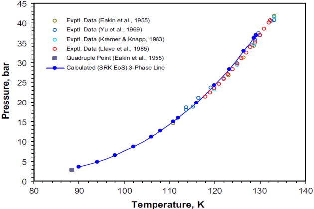
Different authors report slightly different values for the maximum point at which three phases coexistd 133.2 °K and 41.70 bar; 132.38 °K and 40.71 bar; 133.3 °K and 40.74 bar. The system’s quadruple point, at which two liquids, a vapor, and a solid coexist, is also shown in Figure 1 with values as reported by Eakin et al. (1955), namely 88.4 °K and 2.76 bar.
The three-phase experimental data for the system nitrogen + ethane reported by all these authors were used to compare the SRK EoS modeling results.
Figure 1 also shows the agreement between the SRK EoS modeling results and the experimental data of the preceding authors. As can be seen, the maximum three-phase coexisting point predicted with this model is 129.2 °K and 37.03 bar, which is lower both in pressure and temperature than that one determined experimentally.
Figure 2 shows the experimental VLL and SRK EoS predicted equilibrium data on a tem-perature-composition (in terms of nitrogen mole fraction) phase diagram. Though the K-point predicted is lower than the experimental one and the calculated concentrations in the liquid phase \( \style{font-size:22px}{L_2} \) deviate from the experimental concentrations, still the agreement is acceptable. Of course, the liquid compositions calculated can be improved considerably by refitting the binary interaction parameter to the VLE data at each temperature level; that is, adjusting the kij parameter to the VLE data as a function of temperature.

Kremer and Knapp (1983) reported VLE and VLLE data for the nitrogen + ethane system at four temperatures between 120 and 133.15 °K. The experimental data reported by these authors at 120 °K were used to compare the PC-SAFT and SRK modeling results.
Figure 3 shows the experimental data and data calculated with the PC-SAFT and SRK EoSs solubility limits for the nitrogen + ethane system at \( T \) = 120 °K. Both models can reliably predict the \( \style{font-size:22px}{VL\;(V-L_1\;and\;V-L_2)} \) and \( \style{font-size:22px}{V-L_1-L_2} \) solubility limits although the PC-SAFT results are slightly closer to the experimental data. Figure 3 also shows the predicted \( \style{font-size:22px}{L_1-L_2} \) phase equilibria at higher pressures within the solubility limits using both thermodynamic models.

Figure 4 shows details of the nitrogen-rich liquid phase (liquid phase \( \style{font-size:22px}{L_2} \)) in equilibrium with the vapor phase on a pressure-temperature phase diagram. Again, the PC-SAFT performs better than the SRK: at T = 120 °K the experimental \( \style{font-size:22px}{V-L_2} \) composition (in mole fraction) on the three phase line reported by Kremer and Knapp is 0.9398 \( \style{font-size:22px}{N_2} \) (at 23.23 bar), whereas the calculated composition is 0.9632 N2 (at 23.80 bar) and 0.9717 \( \style{font-size:22px}{N_2} \) (at 24.20 bar), respectively.
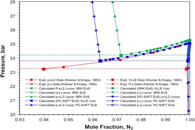
Figure 5 shows the nitrogen + ethane experimental and calculated pressure-temperature phase diagram. The vapor pressure curves for nitrogen and ethane were calculated with the Wagner equation in the “3, 6” form using the parameters reported by Reid et al. (1987); the critical properties for these components are those given in Table 1, and the calculated three-phase VLL line is the one presented in Figure 1.
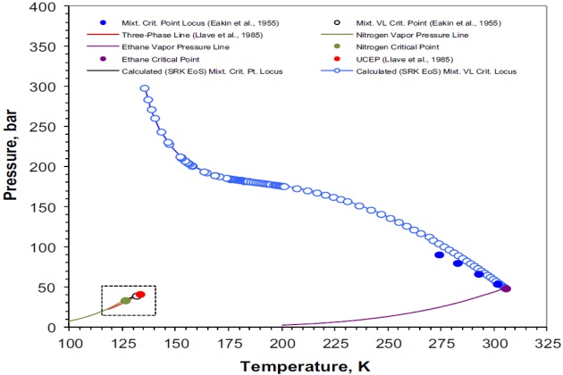
The mixture critical locus shown in Figure 5 was calculated using the procedure presented earlier for locating all the critical points of a given mixture. In this case, the feasible domain to locate all the critical points with the simulated annealing algorithm of Goffe et al. (1994) was defined as a close box in the \( \style{font-size:22px}{T-V} \) plane in the form \( \style{font-size:22px}{\lbrack T_{min},T_{max}\rbrack x\lbrack V_{min},V_{max}\rbrack} \), where the lower and upper limits of temperature \( T \) and volume \( V \) are given by Equations 80 and 81 for one mole of mixture
Figure 5 indicates that \( \style{font-size:22px}{N_{2\;+}} \) ethane is a type III system, according to the classification scheme of van Konynenburg and Scott (1980). Different compositions were studied and it was found that for some the system exhibited more than one critical point. That is, two critical points were found over the \( N_2 \) mole fraction range of [0.6944, 0.6800], one critical point was located within the \( N_2 \) mole fraction ranges of [0.0010, 0.6750] and [0.9995, 0.9600], and no critical point was found over the \( N_2 \) mole fraction range of [0.9500, 0.9700]. The latter case was also experimentally confirmed by Eakin et al. (1955), although they did not report the \( N_2 \) mole fraction range in which there is not any critical point for this binary system.
Figure 6 shows details of the P-T phase diagram of Figure 5 at temperatures between 115 and 135 °K. For the sake of simplicity, this figure presents only the experimental and calculated three- phase VLL line and the UCEP (or K-point).

The vapor pressure for nitrogen is given for reference and it can be seen that both the experimental and calculated VLL loci closely parallel it. It should be noted, however, that the calculated VLL locus is predicted at higher pressures than the experimental one and that the position of the UCEP is found at a temperature and pressure lower than the experimental one. Despite the deviations between the experimentally measured and calculated with the SRK EoS VLL locus and UCEP point, which can be attributed to the binary interaction parameter, this equation gives a satisfactory representation of the experimentally observed phase behavior of nitrogen + ethane system.
The nitrogen + propane system
Schindler (1966) and Schindler et al. (1966) reported VL and LL equilibrium data of 13 isotherms for the nitrogen + propane system from 123.2 to 353.2 °K and pressures ranging up to 137.86 bar. The experimental data reported by these authors show that above 298.2 °K, the critical point of the system was encountered at pressures below 137.86 bar and that at temperatures below 126.7 °K two liquid phases coexist. At a temperature below this value, the system is in vapor-liquid equilibrium up to pressure corresponding to the temperature in question on the three-phase locus.
This system was also studied by Kremer and Knapp (1983) at four isotherms from 120 to 127 °K and pressures up to 62.25 bar, and by Llave et al. (1985) over the temperature range from 117.0 to 126.62 °K and pressures ranging from 21.53 to 34.77 bar. The upper critical end point (K-point) for this binary system reported by Llave et al. (1985) is \( T \) = 126.62 °K and \( p \) = 34:77 bar, which is in a good agreement with the value reported by Schindler et al. (1966) of \( T \) = 126:70 °K and \( p \) = 34.67 bar.
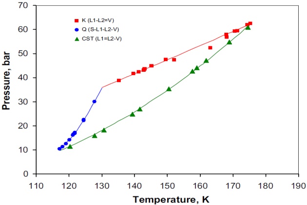
Figure 7 shows on a P-T projection the experimental three-phase VLL locus of the system nitrogen + propane. The calculated three-phase line with the SRK EoS, which is in excellent agreement with the experimental data, is also shown. In this case, the estimated K-point obtained by interpolation of the calculated three-phase line is \( T \) = 126.45 °K and \( p \) = 34.22 bar, which is just slightly lower than the experimental data reported by Schindler et al. (1966) and by Llave et al. (1985). The experimental quadruple point (84.75 °K and 2.27 bar) reported by Schindler et al. (1966) is also shown Figure 7.
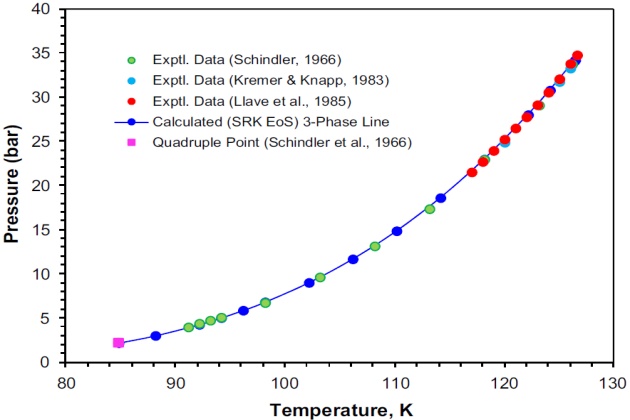
Figure 8 shows on a temperature-composition phase diagram the experimental and calculated (SRK EoS) mole fractions of nitrogen for the two liquid phases \( L_1 \) and \( L_2 \), and the vapor phase \( V \). The calculated liquid phase L1 mole fractions are in very good agreement with the experimental data of Llave et al. (1985). However, the calculated liquid phase \( L_2 \) mole fractions differ slightly from those reported by the same authors. The calculated mole fractions of the liquid phase \( L_2 \) and vapor phase \( V \) are very similar; these two phases are essentially pure nitrogen with concentrations higher than 99 mole %, which become identical at the K-point.
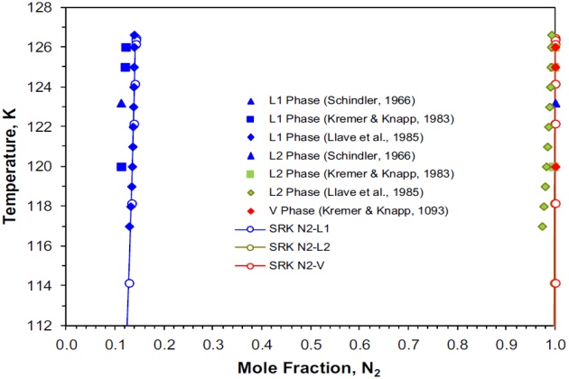
Schindler (1966) reported VLE and LLE data for the nitrogen + propane system at 123.2 °K. As shown in Figure 9, two liquid phases can coexist at this temperature and pressures above 29.09 bar, which is the estimated three-phase VLLE pressure with corresponding \( N_2 \) mole fractions of 0.11150 and 0.99962 for liquid phases \( L_1 \) and \( L_2 \), respectively. At a pressure below this value, the system is in vapor-liquid equilibrium. As noted earlier, liquid phase \( L_2 \) contains only traces of the high boiling component (i.e., propane) and vapor phase is essentially pure nitrogen.
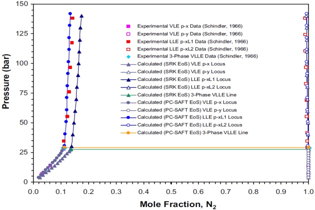
The solubility limits calculated with the SRK and PC-SAFT EoSs are shown in Figure 9. In this case, the PC-SAFT model predicts an VLLE pressure of 29.13 bar with corresponding \( N_2 \) mole fractions of 0.11238 and 0.99996 for liquid phases \( L_1 \) and \( L_2 \), respectively, which is in very good agreement with the estimated “experimental” data.
The calculated three-phase pressure with the SRK model is 27.51 bar with corresponding \( N_2 \) mole fractions of 0.13702 and 0.99921 for liquid phases \( L_1 \) and \( L_2 \), respectively. Although the VLLE pressure and compositions calculated deviate from the experimental data, in general the thermodynamic model predicts satisfactorily the phase behavior of this binary system at low temperatures.
The nitrogen + methane + ethane system
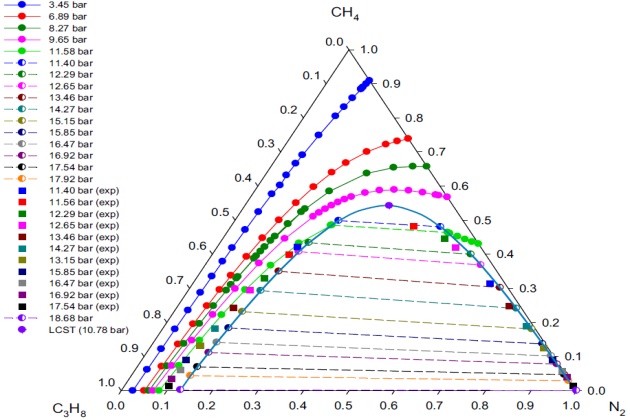
The three-phase VLL region displayed by this ternary system is bounded from above by a K-point locus, from below by a lower critical solution temperature (LCST) locus, while at low temperatures by a Q-point locus. Owing to the fact that the system contains a binary pair (nitrogen + ethane) that exhibits VLL behavior), its VLL space is truncated. In this case, the partially miscible pair nitrogen + ethane spans the VLL space from a position of the LCST locus to a position on the Q-point space. Because methane is of intermediate volatility compared with nitrogen and ethane, it creates a three-phase VLL space that extends from the binary VLL locus upward in temperature. The topographical nature of the regions of immiscibility for the system nitrogen + methane + ethane is shown in Figure 10. In this figure, it can be seen that the \( L-L=V \) and \( L=L-V \) critical end-point loci intersect at a tricritical point \( (L=L=V) \).

Figure 11 shows the good agreement between the experimental and calculated with the PC-SAFT EoS \( L_1-L_2 \) phase behavior of the ternary system at \( T \) = 113.7 °K and different pressures.
An attempt to directly calculate the LCST points at \( T \) = 113.7 °K was carried out by using the procedure described earlier. As pointed out before, the use of good initial guesses, obtained from the VLL calculations close to the LCST, promotes the convergence of the Newton procedure. As a result, the SRK EoS LCST points at 113.7 °K (14.08 bar and 0.5461 \( N_2 \) mole fraction) predictions are completely acceptable (Figure 11). This figure also shows that at pressures away from the LCST point, the PC-SAFT model gives a good representation of the experimental compositions for both liquid phases.
Since there are not experimental data below 15.30 bar at 113.7 °K, a direct comparison of the model with experiment in the region of the LCST is not possible. However, by extrapolation of the experi-mental data, it was possible to determine the pressure of the “hypothetical” experimental LCST at \( T \) = 113:7 °K; that is, \( p≈ \) 15:24 bar. The compositions (in mole fraction) at the LCST were obtained from the experimental tie-lines using the method of Treybal et al. (1946), and they are 0.5660 \( N_2 \), 0.1763 methane, and 0.2577 ethane.
The nitrogen + methane + propane system
This system is topographically similar to the nitrogen + methane + ethane system, sharing the same sort of boundaries: K-point, Q-point, LCST, and binary (nitrogen + propane) VLL loci. Furthermore, the LCST and K-point loci intersect at a tricritical point. However, its three-phase VLL region extends over a much larger area and upward in temperature and pressure from the binary VLL locus in comparison to the nitrogen + methane + ethane system, as shown in Figure 12.
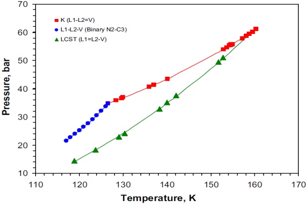
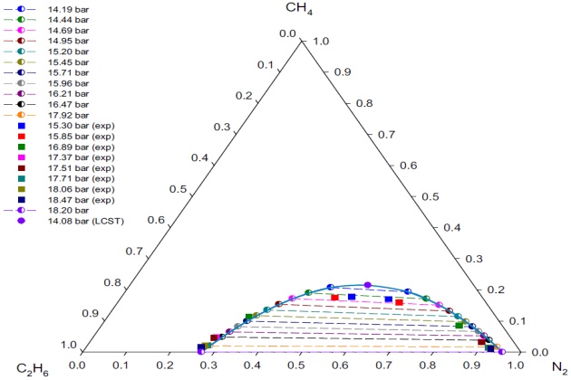
Figure 13 presents the experimental and calculated \( V-L_1-L_2 \) phase behavior (in terms of \( L_1-L_2 \) mole fraction data) for the nitrogen + methane + propane system at \( T \) = 114.1 °K and different pressures. The figure also shows the binodal curve with tie-lines and the LCST calculated. The SRK EoS was used as the thermodynamic model to represent the liquid and vapor phases. Overall, there is a good agreement between the experimental values of \( L_1 \) and \( L_2 \) phases, reported by Poon (1974) and Poon and Lu (1974), and those predicted with the model. It should be noted that the VLL calculations were performed up to almost the position of the binary VLL boundary (\( p \) = 18:68 bar) at \( T \) = 114:1 °K, where methane mole fractions are practically zero in all three phases; that is, this ternary system exhibits LCST but not K-points at this temperature.
At pressures away from the LCST, the SRK EoS gives a reasonable representation of the exper-imental compositions for liquid phase \( L_1 \) (ethane-rich liquid phase) and agrees closely for \( L_2 \) phase (nitrogen-rich liquid phase). The LCST point showed in Figure 13 was determined using the procedure presented earlier for calculating K- and LCST-points. The calculated LCST at 114.1K is 10.78 bar with the following corresponding mole fractions: 0.3176 \( N_2 \), 0.5424 methane, and 0.1400 propane.
Since there are no experimental data below 11.40 bar at 114.1 °K, comparisons of the model with experiment in the region of the LCST are not possible. However, an estimate of the hypothetical experimental LCST was obtained by extrapolating the experimental pressure-composition data of the liquid phases \( L_1 \) and \( L_2 \). The estimated hypothetical experimental pressure at the LCST point is pz11:05 bar. However, due to the scatter of the liquid \( L_2 \) experimental data, it was not possible to use the method of Treybal et al. (1946) to estimate the compositions at the LCST point.
The nitrogen + methane + n-butane system
As mentioned previously, the type of the VLL region displayed by ternary systems depends on whether they contain an immiscible pair or not. In this context, the nitrogen + methane + n-butane system does not exhibit immiscibility in any of their binary pairs. Consequently, the three-phase region displayed by this system is triangular, which is bounded from above by a K-point locus \( (L-L=V) \), from below by a LCST \( (L=L-V) \) locus, and by a Q-point locus \( (S-L-L-V) \) at low temperatures. These three loci intersect at invariant points for this system: the K-point and LCST loci at a tricritical point, whereas the Q-point locus terminates at a point of the type S-L-L=V from above and at a point of the type \( S-L=L-V \) from below, respectively. Figure 14 presents the experimental pressure-temperature diagram of the three-phase VLL space developed by this ternary system. This is a very interesting system because it is in contrast to the other ternary systems examined, which did not exhibit \( L_1-L_2-V \) behavior outside the boundary loci when projected on P-T space. That is, above 150 °K the critical solution temperature (CST) locus is comprised of LCST points, similar to those observed in other nitrogen-containing ternary systems whereas below 150 °K the CST boundary changes to an UCST (upper critical solution temperature) locus, in a manner similar to that exhibited by the systems methane + 2-methylpentane + 2-ethyl-1- butene and methane + 3,3-dimethylpentane + 2-methylhexane reported by van Konynenburg (1968). Figure 14 shows the topographical nature of the regions of immiscibility for the system nitrogen + methane + n-butane. As can be seen, the \( L-L=V \) and\( L=L-V \) critical end-point loci intersect at a tricritical point \( (L=L=V) \).
VLL calculations have been performed at 159.5 °K with both the PC-SAFT and SRK models, where the obtained results are presented in Figure 15. As can be seen, the liquid \( L_1 \) and \( L_2 \) nitrogen mole fractions predicted with the SRK are in a better agreement with the experimental liquid L1 data than those predicted with the PC-SAFT. However, the liquid \( L_2 \) nitrogen mole fractions predicted with both thermodynamic models do not agree well with the experimental data; that is, the SRK underpredicts the experimental data whereas the PC-SAFT overpredicted them. In fact, Figure 15 shows that the PC-SAFT overpredicts both liquid phases. This could be a result of the fact that the interaction parameter of the nitrogen + n-butane binary system for this model was determined at temperatures higher than those studied here.
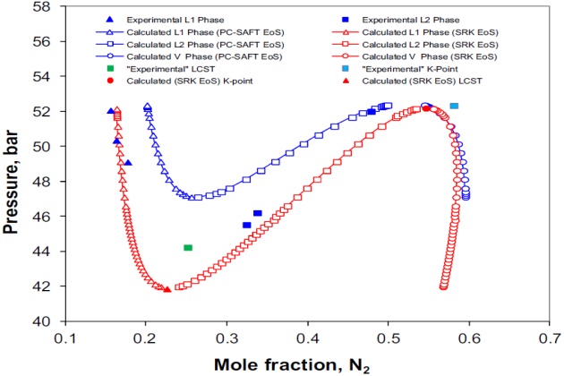
Because at 159.2 °K two critical end pointsda K-point and an LCST dexist on the pressure-tem-perature phase diagram, those were calculated with the SRK model using the aforementioned pro-cedure, which gave a value of 52.20 bar (0.5463 \( N_2 \) mole fraction) and 41.88 bar (0.2256 \( N_2 \) mole fraction) for the K-point and LCST, respectively.
Although there is not any experimental K-point or LCST data for this isotherm, it was possible to estimate it by interpolation. The hypothetical experimental K-point and LCST values reported by Merrill (1983) are, respectively, 52.35 bar (0.5808 \( N_2 \) mole fraction) and 44.25 bar (0.2513 \( N_2 \) mole fraction), and they are also presented in Figure 15. In this case, the experimental K-point and LCST values are, respectively, 0.15 and 2.37 bar above the calculated ones with the SRK model. The esti-mated (by interpolation) K-point and LCST with the PC-SAFT model are 52.39 and 47.11 bar, respectively, which are 0.04 and 2.86 bar above the estimated experimental values, respectively.
The nitrogen + methane + ethane + propane system
Though it has been well recognized that the design of natural gases’ separation processes requires phase equilibrium data, most of the data available in the literature concerns ternary systems. To the best of our knowledge, quaternary vapor-liquid equilibrium data of systems including components of greatest interest to natural gas are limited to the experimental data reported by Trappehl and Knapp (1989).
Trappehl and Knapp present data on the vapor-liquid equilibrium of nitrogen-methane-ethane- propane at 200 °K and pressures from 20 to 120 bar. We model the vapor-liquid equilibria of this system at \( T \) = 200K and \( p \) = 20 bar, applying the SRK EoS as the thermodynamic model. The physical properties of the pure components and the binary interaction parameters required are those given in Tables 1 and 2, respectively.
Figures 16 and 17 depict the calculated compositions against the experimental ones for the liquid and vapor phases, respectively.
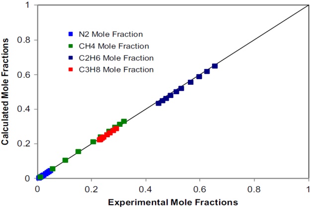
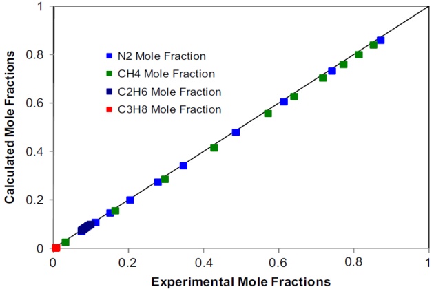
The agreement, in most cases, is quantitative, which demon-strates the capabilities of the SRK EoS to represent the phase behavior of this complex quaternary nitrogen-containing system at low temperatures.
The nitrogen + methane + ethane + propane + n-butane system
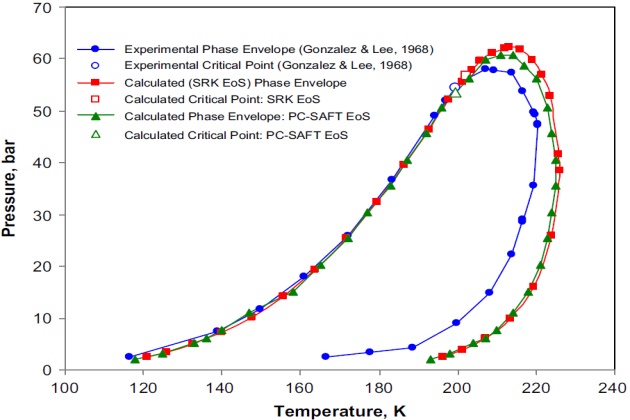
The SRK and PC-SAFT EOSs were applied to predict the phase behavior for this complex quinary LNG mixture experimentally studied by Gonzalez and Lee (1968) in the 116.5 to 220.4 °K temperature range and from 2.4 to 58.0 bar in pressure. The mixture composition reported by these authors is 1.60 mol % \( N_2 \), 94.50 mol % methane, 2.60 mol % ethane, 0.81 mol % propane, and 0.52 mol % butane.
For all calculations, the binary interaction parameters used for the SRK and PC-SAFT EoSs are those of Table 2 for the binaries formed of n-alkanes and \( N_2 \) with n-alkanes.
The phase behavior predictions obtained with the SRK and PC-SAFT EoSs are displayed in Figure 18. As can be observed the calculated two-phase envelopes exhibit a wide retrograde zone. This was verified with direct critical point calculations performed with the SRK (202.2K and 56.78 bar) and PC-SAFT (199.5 °K and 53.63 bar) models by using the procedures presented by Justo-Garcla et al. (2008a,b). For the SRK model, the simulated annealing algorithm was used for solving the criticality conditions based on the tangent plane distance in terms of the Helmholtz energy using temperature and volume as independent variables, whereas for the PC-SAFT model, the mixture critical point calculation was carried out by using the algorithm of Heidemann and Khalil (1980). In both cases, the calculations showed that this mixture presents a single gas-liquid critical point on the two-phase boundary, which is consistent with the experimental critical point (199.5 °K and 54.57 bar) reported by Gonzalez and Lee (1968).
The calculated phase envelopes (Figure 18) were constructed applying the two procedures presented earlier.
Furthermore, Figure 18 shows the good agreement between the experimentally measured and calculated bubble-point curves, while the calculated dew-point curves with both models are very similar to but less satisfactory than the experimental data. Notwithstanding, it is worth mentioning that since the interaction parameters for the SRK and PC-SAFT models were determined from binary vapor-liquid equilibrium data, the rather poor fit in this region with either model is not unexpected.
Further examination of Figure 18 indicates a regular sequential consistent behavior of the phases at equilibrium for this mixture. That is, at low pressures, on the dew-point curve side, only a single stable vapor phase exists. Insofar as pressure increases, the liquid phase appears and the mixture becomes stable as vapor-liquid. At higher pressures, the liquid disappears and the mixture becomes stable as vapor.