In-Depth Exploration of Airy Functions and Their Applications

Uncover the intricacies of Airy functions in this detailed guide, featuring clear definitions, asymptotic formulas for large arguments, and their critical role in the diffraction and scattering of UHF waves.

СодержаниеСвернуть

Definitions
Asymptotic Formulas for Large Arguments
Integrals Containing Airy Functions in Problems of Diffraction and Scattering of UHF Waves
Integral V₁
Integral V₂
Integral V₄
Integral V₅

Explore specific integrals, including V1, V2, V4, and V5, to gain a deeper understanding of their applications in various scientific and engineering contexts.

Definitions

Studying the behavior of light in the neighbourhood of caustics in 1838, Sir G. B. Airy introduced the famous integral:

ν (t) = \frac{1}{\sqrt{π}} \int_{0}^{\infty} \cos (\frac{x^{3}}{3} + x t) d x E q . 1

which represents one of the solutions to the differential equation:

w^{''} (t) - t w (t) = 0, E q . 2

namely, one which decreases at positive infinity more rapidly than any finite power of t. A second independent solution to Eq. (2) can be named u(t) and will be defined later.

Following Fock, the solution to Eq. (2) can also be defined via the integral:

w (t) = \frac{1}{\sqrt{π}} \int_{Γ_{1}} d z \exp (t z - \frac{z^{3}}{3}) E q . 3

where contour Γ₁ goes by the ray with arg z = -2π/3 from infinity to 0 and then to infinity along the real and positive z-axis, Figure 1.

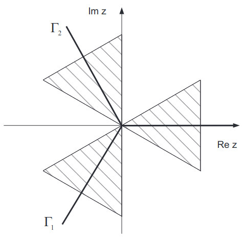
Fig. 1 Sectors of convergence for the Airy integral

Consider the behavior of the function w(t) with real argument t. First, let us find the sector of convergence of the integral (3) in order to perform useful deformations on the integration contour. With |z| → ∞ we may neglect the first term in the integrand (3) then the convergence sector is determined by the condition:

Re z^{3} > 0 . E q . 4

We may define z = |z|e^jα(-π < α < π), then the condition (4) results in:

\cos (3 α) > 0, E q . 5

which, in turn, determines three sectors of convergence of the integral (3) in the z-plane:

1) - \frac{π}{6} < α < \frac{π}{6},

2) \frac{π}{2} < α < \frac{5 π}{6}, E q . 6

3) - \frac{5 π}{6} < α < - \frac{π}{2} .

The contour Γ₁ in Eq. (3) passes through the middle of the first and the third sector and therefore coincides with one of the lines of steepest descent of the integrand’s phase.

We can now deform the contour Γ₁ within the sector of convergence without changing the value of the integral. Let us turn the lower part of contour Γ₁ to coincide with the negative imaginary axis of z. Then integral (3) can be written in the following form:

w (t) = \frac{1}{\sqrt{π}} \int_{0}^{\infty} d z \exp (t z - \frac{z^{3}}{3}) + \frac{1}{\sqrt{π}} \int_{- j \infty}^{0} d z \exp (t z - \frac{z^{3}}{3}) . E q . 7

Changing the variable in the second integral (7) to ς = jz, we obtain:

w (t) = \frac{1}{\sqrt{π}} \int_{0}^{\infty} d z {\exp (t z - \frac{z^{3}}{3}) + \frac{j}{\sqrt{π}} \int_{0}^{\infty} d ς \exp (- j (t ς - \frac{ς^{3}}{3})) . E q . 8

We may nowselect the real and imaginary parts in w(t):

w (t) = u (t) + j ν (t) . E q . 9

where:

u (t) = \frac{1}{\sqrt{π}} \int_{0}^{\infty} d z \exp (t z - \frac{z^{3}}{3}) + \frac{1}{\sqrt{π}} \int_{0}^{\infty} d z \sin (t z + \frac{z^{3}}{3}), E q . 10

ν (t) = \frac{1}{\sqrt{π}} \int_{0}^{\infty} d z \cos (t z + \frac{z^{3}}{3}) = \frac{1}{2 \sqrt{π}} \int_{0}^{\infty} d z \exp (- j (t z + \frac{z^{3}}{3})) . E q . 11

As observed from Eqs. (9) to (11), functions u(t) and ν(t) represent two independent solutions to Eq. (2), and ν(t) is indeed an original Airy integral (1). The functions u(t) and ν(t) are related via the following equation:

u^{'} (t) ν (t) - u (t) ν^{'} (t) = 1 . E q . 12

The set of two independent solutions to Eq. (2) can also be found in terms of another contour integral of Eq. (2). Further we redefine the first integral (3) as a function w₁(t) while the second integral we define in the following form:

w (t) \equiv w_{2} (t) = \frac{1}{\sqrt{π}} \int_{Γ_{2}} d z \exp (t z - \frac{z^{3}}{3}) . E q . 13

The contour Γ₂ is a mirror image of the contour of Γ₁ relative to the real axis of z shown by the dashed line in Figure 1. With real values of the arguments, functions w₁(t) and w₂(t) are complex conjugate and:

w_{2} (t) = u (t) - j ν (t) . E q . 14

For functions w2(t) and w1(t) there exists an equation similar to Eq. (10):

w_{1}^{'} (t) w_{2} (t) - w_{2}^{'} (t) w_{1} (t) = - 2 j E q . 15

and:

w_{1} (t e^{j 2 π / 3}) = e^{j π / 3} w_{2} (t) . E q . 16

While functions u(t) and ν(t) are real functions with real values of the argument t, these are also natural transcendent functions valid for complex values of t. The relations (9) and (14) hold for complex t. Numerous formulas, useful for the treatment of Airy functions, have been provided by Fock and some of them are listed below for convenience:

w_{1} (t e^{j π / 3}) = 2 e^{j π / 6} ν (- t), E q . 17

w_{1} (t e^{j π}) = u (- t) + j ν (- t), E q . 18

w_{1} (t e^{j 4 π / 3}) = 2 e^{j π / 6} ν (t), E q . 19

w_{1} (t e^{j 5 π / 3}) = e^{j π / 3} [u (- t) - j ν (- t)] . E q . 20

The above relations represent the values of the function w₁(t) at the rays arg t = nπ/3 (n = 0, 1, 2, 3, 4, 5) in the complex t-plane via real functions u(t) and ν(t) with real values of the argument t.

We may also note that the functions u(t) and ν(t) are equivalent to Airy functions Ai(t) and Bi(t):

A i (t) = \frac{1}{\sqrt{π}} ν (t); B i (t) = \frac{1}{\sqrt{π}} u (t) .

Asymptotic Formulas for Large Arguments

The asymptotic expressions for the Airy function for large arguments have been derived by Fock and are provided below. Frequently used formulas for large negative t are:

w_{1} (t) = {(- t)}^{- 1 / 4} \exp [j \frac{2}{3} {(- t)}^{3 / 2} + j \frac{π}{4}], E q . 21

w_{2} (t) = {(- t)}^{- 1 / 4} \exp [- j \frac{2}{3} {(- t)}^{3 / 2} - j \frac{π}{4}], E q . 22

Let us introduce the definition:

x = \frac{2}{3} t^{3 / 2}

and coefficients a_n, b_n to be used in the forthcoming formulas:

a_{1} = \frac{5}{72}; a_{2} = \frac{(5 \cdot 11) \cdot 7}{1 \cdot 2 \cdot {(72)}^{2}}; a_{3} = \frac{(5 \cdot 11 \cdot 17) \cdot (7 \cdot 13)}{1 \cdot 2 \cdot 3 {(72)}^{3}};

a_{n} = \frac{(5 \cdot 11 . . . (6 n - 1)) \cdot (7 \cdot 13 . . . (6 n - 5))}{1 \cdot 2 \cdot . . . n {(72)}^{n}},

b_{1} = \frac{7}{72}; b_{2} = \frac{(7 \cdot 13) \cdot 5}{1 \cdot 2 \cdot {(72)}^{2}}; b_{3} = \frac{(7 \cdot 13 \cdot 19) \cdot (5 \cdot 11)}{1 \cdot 2 \cdot 3 \cdot {(72)}^{3}};

b_{n} = \frac{(7 \cdot 13 . . . (6 n + 1)) \cdot (5 \cdot 11 . . . (6 n - 7))}{1 \cdot 2 \cdot . . . n {(72)}^{n}} .

Then a comprehensive asymptotic expression for Airy functions of large positive argument t can be written as follows:

u (t) = t^{- 1 / 4} e^{x} (1 + \frac{a_{1}}{x} + \frac{a_{2}}{x^{2}} + . . .), E q . 23

u^{'} (t) = t^{1 / 4} e^{x} (1 - \frac{b_{1}}{x} - \frac{b_{2}}{x^{2}} - . . .), E q . 24

ν (t) = \frac{1}{2} t^{- 1 / 4} e^{- x} (1 - \frac{a_{1}}{x} + \frac{a_{2}}{x^{2}} - \frac{a_{3}}{x^{3}} + . . .), E q . 25

ν^{'} (t) = - \frac{1}{2} t^{1 / 4} e^{- x} (1 + \frac{b_{1}}{x} - \frac{b_{2}}{x^{2}} + \frac{b_{3}}{x^{3}} - . . .), E q . 26

For large negative t we have:

u (- t) = t^{- 1 / 4} \cos (x + \frac{π}{4}) (1 - \frac{a_{2}}{x^{2}} + \frac{a_{4}}{x^{4}} - \frac{a_{6}}{x^{6}} + . . .) + t^{- 1 / 4} \sin (x + \frac{π}{4}) (\frac{a_{1}}{x} - \frac{a_{3}}{x^{3}} + \frac{a_{5}}{x^{5}} - \frac{a_{7}}{x^{7}} + . . .), E q . 27

u^{'} (- t) = t^{1 / 4} \sin (x + \frac{π}{4}) (1 + \frac{b_{2}}{x^{2}} - \frac{b_{4}}{x^{4}} + \frac{b_{6}}{x^{6}} - . . .) + t^{1 / 4} \cos (x + \frac{π}{4}) (\frac{b_{1}}{x} - \frac{b_{3}}{x^{3}} + \frac{b_{5}}{x^{5}} - \frac{b_{7}}{x^{7}} + . . .), E q . 28

ν (- t) = t^{- 1 / 4} \sin (x + \frac{π}{4}) (1 - \frac{a_{2}}{x^{2}} + \frac{a_{4}}{x^{4}} - \frac{a_{6}}{x^{6}} + . . .) - t^{- 1 / 4} \cos (x + \frac{π}{4}) (\frac{a_{1}}{x} - \frac{a_{3}}{x^{3}} + \frac{a_{5}}{x^{5}} - \frac{a_{7}}{x^{7}} + . . .), E q . 29

ν^{'} (- t) = t^{1 / 4} \cos (x + \frac{π}{4}) (1 + \frac{b_{2}}{x^{2}} - \frac{b_{4}}{x^{4}} + \frac{b_{6}}{x^{6}} - . . .) + t^{1 / 4} \sin (x + \frac{π}{4}) (\frac{b_{1}}{x} - \frac{b_{3}}{x^{3}} + \frac{b_{5}}{x^{5}} - \frac{b_{7}}{x^{7}} + . . .), E q . 30

Integrals Containing Airy Functions in Problems of Diffraction and Scattering of UHF Waves

In this section we obtain the asymptotical expansions of the integrals containing the product of the Airy–Fock functions:

V = \int_{- \infty}^{0} w (t - γ) w (t - γ_{0}) e x p (j ξ t) d t E q . 31

where w(x) is any one of the solutions to the Airy equation:

w^{'} (x) - x w (x) = 0 E q . 32

defined by one of the integrals below with desirable behavior at infinity:

w (x) \equiv w_{1} (x) = \frac{1}{\sqrt{π}} \int_{Γ} d z \exp (x z - \frac{z^{3}}{3}), E q . 33

w_{1} {(x)}_{x \to \infty} ~ {(- x)}^{- 1 / 4} \exp [j \frac{2}{3} {(- x)}^{3 / 2} + j \frac{π}{4}], E q . 34

w (x) \equiv ν (x) = \frac{1}{2 \sqrt{π}} \int_{- \infty}^{\infty} d z \exp [j \frac{z^{3}}{3} + j z x], E q . 35

ν {(x)}_{x \to \infty} ~ {(x)}^{- 1 / 4} \exp [- \frac{2}{3} {(x)}^{3 / 2}] . E q . 36

In integral (33) the contour Γ elapses from ∞ along the ray exp (j 4π/3) towards 0 and then along the real axis of z to + ∞. Figure 1. Along with the functions w₁(x), ν(x) we use function w₂(x) = w₁^*(x), where the sign * denotes complex conjugate.

Integrals of type (31) are often calculated in problems of UHF diffraction and propagation in the atmospheric boundary layer. This is because in an analytical approach the model of the average refractivity can be described in terms of the linear approximation to a whole height profile of the averaged refractivity or, at least, to some sections of the profile. For instance, the integral of type (31) appears when one need coefficients of the energy transformation between modes (coupling coefficients) due to scattering on the random fluctuations of the refractive index in the medium. Then the eigenfunctions of the operator:

L_{z} [φ_{z}] = [\frac{d^{2}}{d z^{2}} - k^{2} (ε_{0} - g_{ε} z)] φ_{n} (z) = E_{n} φ_{n} (z), E q . 37

φ_{n} (z = 0) = 0, φ_{n} (z \to \infty) = 0 E q . 38

associated with the discrete spectrum of eigenvalues correspond to the waves propagating with almost negligible attenuation, i. e. waveguide modes (trapped modes in the common terminology of tropospheric duct propagation). In the case of linear profile ε(z) these functions can be expressed via the Airy function:

φ_{n} (z) = C_{n} ν (\frac{E_{n} - μ^{3} (z - H)}{μ^{2}}) E q . 39

where z is the height above the boundary surface (z = 0), μ³ = ag_ε/2 the gradient of the refractive index inside the waveguide, i. e. for 0 < z < H, H the thickness of the waveguide formed by a negative gradient of the refractive index g_ε, g_ε = -(dε/dz+2/a).

The coefficient of re-scattering V_m,n between the modes with numbers m and n due to scattering on a spatial Fourier-component of the fluctuation in the refractive index with vertical wavenumber κ is then given by:

V_{m, n} (κ) = \int_{0}^{\infty} d z ν (\frac{E_{n} - μ^{3} (z - H)}{μ^{2}}) ν (\frac{E_{m} - μ^{3} (z - H)}{μ^{2}}) \exp (j κ z) . E q . 40

After apparent transformations, the evaluation of integral (40) will result in calculation of the integral:

V_{1} = \int_{0}^{\infty} d t \cdot ν (t - ξ_{n}) ν (t - ξ_{m}) \exp (j q t) . E q . 41

Similar arguments can be applied to evaluation of the coupling coefficients of the eigenfunctions of the continuous spectrum Ψ_E₁(z) and Ψ_E₂(z). These coefficients will result in integrals of the following kind:

V_{2} = \int_{- \infty}^{0} d t \cdot w_{1} (t - ξ_{1}) w_{1} (t - ξ_{2}) \exp (j q t), E q . 42

V_{3} = \int_{- \infty}^{0} d t \cdot w_{1} (t - ξ_{1}) ν (t - ξ_{2}) \exp (j q t), E q . 43

V_{4} = \int_{- \infty}^{0} d t \cdot w_{1} (t - ξ_{1}) w_{2} (t - ξ_{2}) \exp (j q t) = J_{1} - 2 j J_{3} . E q . 44

We can note that:

V_{5} = \int_{- \infty}^{0} d t \cdot w_{2} (t - ξ_{1}) w_{2} (t - ξ_{2}) \exp (j q t) = J_{2} (- q, ξ_{1}, ξ_{2}) E q . 45

for real q, ξ₁ and ξ₂. Therefore, the basic set of integrals of interest is J₁, J₂ andJ₃.

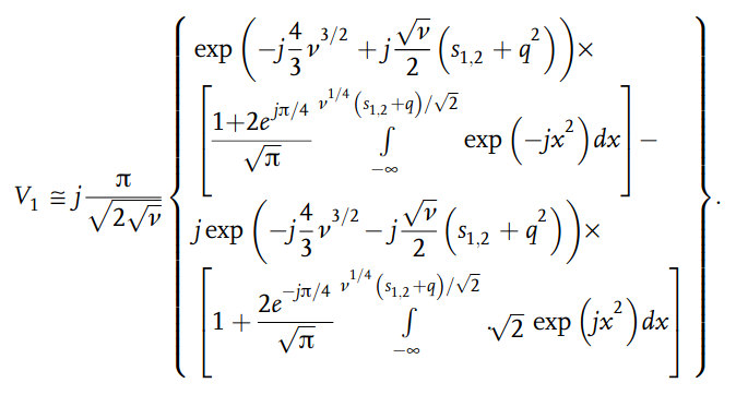
Integral V₁

Making use of the integral representation (35), transform integral V₁ into a triple integral and perform integration over the variable t as well as over one of the newly introduced variables of integration. As a result we obtain:

V_{1} = \frac{\exp (j^{π / 4})}{4 \sqrt{π}} \int_{- \infty}^{\infty} \frac{d s}{\sqrt{s} (s + q)} \exp (j \frac{s^{3}}{12} - j s ν - j \frac{δ}{4 s}) E q . 46

where the contour of integration over s encircles the singularities s = 0 and s = q in the upper half-plane of the variable s; ν = (ξ₁+ξ₂)/2, δ = ξ₁-ξ₂. With |ν| ≫ 1 integral (46) can be calculated using the method of stationary phase.

Assume ν ≫ 1, δ ≫ 1. In the integral (1.1) we observe four stationary points:

S_{1, 2, 3, 4} = \pm (\sqrt{ξ_{1}} \pm \sqrt{ξ_{2}}) .

The pair:

S_{3, 4} = \pm (\sqrt{ξ_{1}} - \sqrt{ξ_{2}}) \approx \pm \frac{δ}{2 \sqrt{ν}}

may come close to the square root singularity in the point s = 0. Let us evaluate the contribution of the stationary points:

S_{1, 2} = \pm (\sqrt{ξ_{1}} + \sqrt{ξ_{2}}) \approx 2 \sqrt{ν} (1 - \frac{δ^{2}}{32 ν^{2}}) .

We may notice that:

V_{1} = \frac{\exp (- j^{π / 4})}{4 \sqrt{π}} (I_{1} (ν, δ, q) + j I_{1}^{*} (ν, δ, - q)), E q . 47

where:

I_{1} = \int_{0}^{\infty} \frac{d s}{\sqrt{s} (s + q)} e x p (j \frac{s^{3}}{12} - j s ν - j \frac{δ}{4 s}) . E q . 48

With

\frac{δ}{2 \sqrt{ν}} ≪ 1 :

I_{1} (ν, δ, q) ≅ I_{1} (ν, 0, q) = \frac{\exp (j^{4 / 3} ν^{3 / 2})}{\sqrt{2 \sqrt{ν}}} \int_{- \infty}^{\infty} \frac{d x}{(x + 2 \sqrt{ν} + q)} \exp (j \frac{s^{3}}{2} - j s ν - j \frac{δ}{4 s}) E q . 49

Taking into account the known representation for the error integral, we obtain:

I_{1} (ν, δ, q) ≅ - j \frac{π}{\sqrt{2 \sqrt{ν}}} \{1 + \frac{2}{\sqrt{π}} \exp (j \frac{π}{4}) \int_{- \infty}^{ν^{1 / 4} (s_{1} + q) / \sqrt{2}} d x \exp (- j x^{2})\} E q . 50

and, respectively, a uniform asymptotic for the contribution to J₁ from stationary points

s_{1, 2} = \pm 2 \sqrt{ν} :

Now, let us evaluate the contribution to V₁ of the region in the vicinity of the stationary points

s_{3, 4} \approx \pm δ / 2 \sqrt{ν} .

We may notice that with

δ ≫ 2 \sqrt{ν}

evaluation of the integral can be performed similarly to the method used in obtaining Eq. (51). Therefore, attention will be paid to the case

δ ≪ 2 \sqrt{ν},

which, being applied to the problem of scattering on random fluctuations in the refractive index, corresponds to the situation where the transversal wavenumbers of the mode’s pair are large, though the distance between the modes in a wavenumber space is small. This situation occurs in a multimode tropospheric duct for higher-order modes when the duct is formed, for instance, by inversion of temperature.

Taking into account that the major contribution to the integral comes from the region of small s, s ~ 1/ν, we may expand exp (js³/12) into a Taylor series:

V_{1} ≅ - \frac{e^{- j π / 4}}{4 \sqrt{π}} \int_{- \infty}^{\infty} d s \frac{\exp (- j s ν - j \frac{δ^{2}}{4 s})}{\sqrt{s} (s + q)} (1 + j \frac{s^{3}}{12} - j \frac{s^{9}}{288} + . . .) = \frac{e^{j π / 4}}{4 \sqrt{π}} [I_{2} (ν, δ, q) + \frac{1}{12} \frac{\partial^{3}}{\partial ν^{3}} I_{2} (ν, δ, q) + . . .] . E q . 52

We may observe that:

I_{2} = e^{j ν q} I_{3}; I_{3} = \int_{- \infty}^{\infty} d s \frac{\exp (- j ν (s + q) - j \frac{δ^{2}}{4 s})}{\sqrt{s} (s + q)} . E q . 53

Now, introduce a new function I₄ using the relation:

I_{4} = \frac{\partial I_{3}}{\partial ν} j e^{j ν q} . E q . 54

The function I₄ is then determined via the integral:

I_{4} = \int_{0}^{\infty} \frac{d s}{\sqrt{s}} [\cos (ψ (s, ν, δ)) + \sin (ψ (s, ν, δ))] E q . 55

where ψ(s, ν, δ) = νs+δ/4s. The integral (55) is tabulated and given by:

I_{4} = \sqrt{\frac{2 π}{\sqrt{ν}}} \cos (δ \sqrt{ν}) .

Then, the reverse operation leads to:

I_{2} = 2 \sqrt{π} e^{- j 3 π / 4 + j ν q} \int_{\infty}^{ν} d η e^{j η q} \frac{\cos (δ \sqrt{η})}{\sqrt{η}} + C . E q . 56

The value of constant C, which does not depend on parameter q, can be chosen using the norm of J₁ with q → 0. Then:

C = j \frac{2 π}{\sqrt{q}} \exp (j \frac{δ^{2}}{4 q} - j \frac{π}{4}) .

After some transformation expression for I₂ the following results:

I_{2} (ν, δ, q) = - \frac{2 \sqrt{π}}{\sqrt{q}} \exp (- j \frac{3 π}{4} + j ν q + j \frac{δ^{2}}{4 q}) \cdot \{\erf [e^{j π / 4} (\sqrt{q} ν - \frac{δ}{2 \sqrt{q}})] + \erf [e^{j π / 4} (\sqrt{q} ν + \frac{δ}{2 \sqrt{q}})]\} E q . 57

where erf(.) is the error integral.

It should be noted that the second term in Eq. (52) has an order O(1/ν^3/2) and may be neglected for the following reason. We seek the estimate of the integral J₁ as a sum of Eqs. contributions from the stationary points, four in total. Therefore, the result is a combination of (51) and (52).

Taking into account that the contribution of the stationary points

s_{1, 2} = \pm 2 \sqrt{ν}

in Eq. (51) evaluated with precision up to the terms of order

O (1 / \sqrt{ν})

, we should neglect the second term in Eq. (52), thus substituting the expression (57) for I₂ in Eq. (52).

Finally with ν ≫ 1, δ ≪ 1, the integral V1 m; d; qð Þ is represented by a sum of contributions of four stationary points:

V_{1} (ν, δ, q) \approx {V_{1}}_{s = s_{1}} + {V_{1}}_{s = s_{21}} + {V_{1}}_{s = s_{3}} + {V_{1}}_{s = s_{4}},

where

{V_{1}}_{s = s_{1}}

and

{V_{1}}_{s = s_{2}}

are defined by Eq. (51) and

{V_{1}}_{s = s_{3}}

and

{V_{1}}_{s = s_{4}}

by Eqs. (52) and (57).

In the limiting case δ = 0 and qν ≪ 1 we obtain:

V_{1} (ν, δ, q) = \sum_{p = 0}^{\infty} \frac{2^{p} e^{j π p / 2}}{(2 p + 1)} q^{p} ν^{p + 1 / 2} + O (\frac{1}{\sqrt{ν}}) . E q . 58

With q = 0, ν = ξ_n (recall that ξ_n is a propagation constant of the nth mode), the expression (58) equates to the known asymptotic of the norm of the eigenfunctions of the discrete spectrum with ξ_n ≫ 1:

N_{n} = \int_{0}^{\infty} d t ν^{2} (t - ξ_{n}) = \sqrt{ν} . E q . 59

a) Let us consider the integral J₁ with small parameters δ, ν: ν ≪ 1, δ ≪ 1. Expanding exp(-jνs-jδ²/4s) and (s+q)^-1 into a series, we obtain:

V_{1} (ν, δ, q) = \sum_{m = 0}^{\infty} \sum_{p = 0}^{\infty} \sum_{r = 0}^{\infty} B_{p m r} \frac{{(- 1)}^{r} e^{- j π p + m / 2}}{p! m! 2^{2 m}} q^{r} ν^{p} E q . 60

where:

B_{p m r} = {(12)}^{\frac{m - p + r}{3}} Γ (\frac{p - m + r}{3} - \frac{1}{6}) \cdot [\exp (j \frac{π}{6} (p - m - r - \frac{1}{2})) + \exp (j \frac{5 π}{6} (p - m - r - \frac{1}{2}))] .

In the particular case when q = ν = δ = 0, integral (15) equates to:

V_{1} = \frac{Γ (\frac{5}{6}) 2^{- 4 / 3}}{\sqrt{π} 3^{1 / 6}} E q . 61

which is the same as the known integral:

\int_{0}^{\infty} d x ν^{2} (x) = {[- \frac{\sqrt{π}}{3^{1 / 3} Γ (\frac{1}{3})}]}^{2} = \frac{Γ (\frac{5}{6}) 2^{- 4 / 3}}{\sqrt{π} 3^{1 / 6}} . E q . 62

b) With qν ≫ 1 we may expand (s+q)^–1 over the reverse powers of q thus obtaining the series representation:

V_{1} (ν, δ, q) = \sum_{m = 0}^{\infty} \sum_{p = 0}^{\infty} \sum_{r = 0}^{\infty} B_{p m r} \frac{{(- 1)}^{r} e^{- j π p + m / 2}}{p! m! 2^{2 m}} \frac{ν^{p} δ^{2 m}}{q^{r + 1}} E q . 63

where:

B_{p m r} = {(12)}^{\frac{m - p + r}{3} - \frac{1}{6}} Γ (\frac{p - m + r}{3} - \frac{1}{6}) \cdot [\exp (j \frac{π}{6} (p - m - r + \frac{1}{2})) + \exp (j \frac{5 π}{6} (p - m - r + \frac{1}{2}))] . E q . 64

c) When ν ~ 1, δ ≪ 1, we may expand exp(jsν+j δ/4) over a series of Bessel functions, thus obtaining:

V_{1} (ν, δ, q) = \sum_{m = - \infty}^{\infty} {(- j)}^{m} J_{m} (δ \frac{\sqrt{ν}}{2}) {(\frac{2 \sqrt{ν}}{δ})}^{m} B_{m} (q) E q . 65

where J_m(x) is a Bessel function of the first kind and coefficient B_m(q) is given by the integral:

B_{m} (q) = \int_{- \infty}^{+ \infty} d s \frac{\exp (j \frac{s^{3}}{12})}{s + q} s^{m - \frac{1}{2}}, E q . 66

which can be represented via Gamma-functions similar to the coefficient in Eqs. (61) and (64).

Integral V₂

Let us consider integral (42) where ξ₁ and ξ₂ have real and positive values, q is a parameter of real value:

V_{2} = \int_{- \infty}^{0} d t \cdot w_{1} (t - ξ_{1}) w_{1} (t - ξ_{2}) \exp (j q t)

We use the integral representation for Airy functions (33) to transform the integral (42). The contour of the integration Γ₁ in (33) can be defined as elapsing from -j∞ to 0 and then to ∞ along the real axis. After integration over variable t we obtain:

V_{2} = \frac{1}{π} \int_{Γ} \int_{Γ} d ς_{1} d ς_{2} \frac{\exp (- ξ_{2} ς_{1} - ξ_{1} ς_{2} - \frac{ς_{1}^{3} + ς_{2}^{3}}{3})}{ς_{1} + ς_{2} + σ + j q} . E q . 67

We have introduced an additional small parameter σ, σ > 0, in order to shift the pole from the contour of integration into point -(σ+jq) and make a transformation of the contour Γ₁ into contour

Γ_{1}^{'}

as shown in Figure 2.

Integral V2 — Fig. 2 Contour of integration for integral V₂

Introducing a newvariable s = ς₁+ς₂ and redefining for convenience ς ≡ ς₁, we may find that integration over variable ς can then be performed given the convergence after changing the order of integration:

V_{2} = \frac{1}{\sqrt{π}} \int_{Γ_{2}} d s \frac{\exp (- \frac{s^{3}}{12} - s \frac{ξ_{1} + ξ_{2}}{2} + \frac{{(ξ_{1} - ξ_{2})}^{2}}{4 s})}{\sqrt{s} (s + j q + σ)} . E q . 68

The contour Γ₂ for the newly introduced variable s can be obtained from contour Γ₁ by shifting Γ₁ to a value ς₂. When ς₂ varies along the imaginary axis, the contour Γ₁ is shifted down along that axis to ς₂. When ς₂ ≥ 0, the contour Γ₁ should be shifted right along the real axis, i. e. contour Γ₂ of the integration over s seems to depend on the value of ς₂. We may demonstrate that all these variations in contour Γ₂ are equivalent to contour Γ₁.

Consider first the case, when the contour Γ₁ is shifted along the imaginary axis s to the value -|ς₂| as shown in Figure 3.

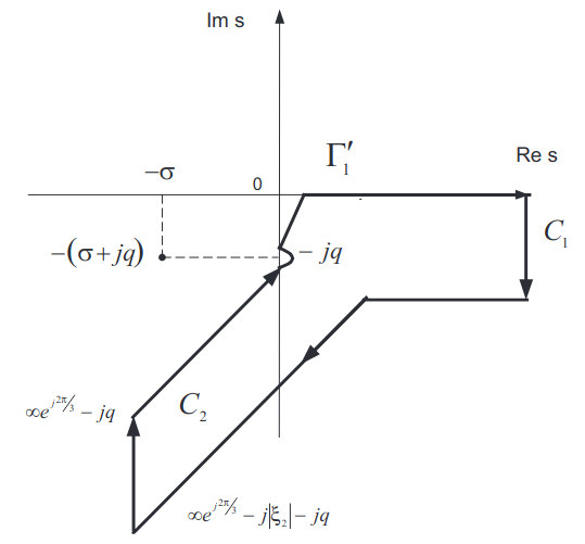
Integration contour — Fig. 3 Transformation of the integration contour in V₂

Inside the closed contour in Figure 3, integral V₂ has no singularities and along the branches C₁ and C₂ of the contour its magnitude is negligible. Therefore, according to Cauchy’s theorem, we may perform integration over contour Γ₁ instead of Γ₂, i. e. these contours are equivalent in terms of integration.

Using similar arguments we may show that when the contour Γ₂ is obtained by a shift of Γ₁ along the real axis, both contours are equivalent. Therefore, whatever value ς₂ takes along contour Γ, contour Γ₂ can be deformed into contour Γ₁ which, in turn, no longer depends on value ς₂, thus allowing, in principle, the changes in the order of integration in Eq. (68).

In order to perform the integration we need to deform the contours Γ and Γ₂ within their sector of convergence in such a way that will ensure convergence of the integral over variable ς. New contours will have the following shape: contour Γ goes from negative ∞ along the ray e^-j2π/3 to 0 and then along the real axis to ∞; contour Γ₂ goes from -j∞ to 0 overtaking the pole –jq from the right (in a counter clockwise direction) and then to ∞ along the ray e^-jπ/6.

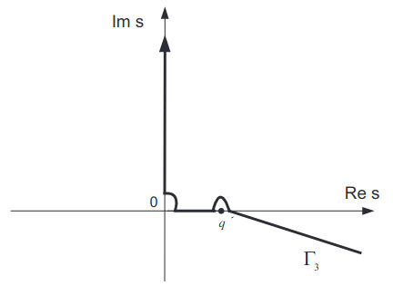
The internal integral over ς is then a Poisson’s integral with apparent solution. In the remaining single integral we then make a further transformation of the contour of integration Γ₂, namely we can turn the contour Γ₂ through an angle of π/2 in a counterclockwise direction and change the path along the contour in the opposite direction, then parameter σ can be put to 0.

Finally, we end up with the following integral:

V_{2} = - \frac{e^{j \frac{π}{4}}}{\sqrt{π}} \int_{Γ_{3}} d s \frac{\exp (- j \frac{s^{3}}{12} + j s ν - j \frac{δ^{2}}{4 s})}{\sqrt{s} (s - q)} E q . 69

with contour Γ₃ shown in Figure 4.

Now we can evaluate integral (69) in some limiting cases.

a) Consider the case when ν ≫ 1, δ ≪ 1.

The integrand in Eq. (69) along the imaginary axis represents a rapidly attenuating function without any singularities at that section of integration. The major contribution to Eq. (69) hence follows from the integration along the ray e^-jπ/6 (or along the real axis of s, since that section of the contour Γ₃ can be further transformed to one along the real axis).

The asymptotic evaluation of the integral (69) is then composed of a contribution from the stationary points:

$s_{1} = 2 \sqrt{ν} (1 - δ^{2} / 32 ν);$
$s_{3} = δ / 2 \sqrt{ν} :$

V_{2} \approx {V_{2}}_{s_{1}} + {V_{2}}_{s_{3}} E q . 70

where:

{V_{2}}_{s_{1}} ≅ - \frac{e^{j π / 4}}{\sqrt{π}} I_{5} (ν, δ, q) E q . 71

and:

I_{5} (ν, δ, q) = \int_{0}^{\infty} d s \frac{\exp (- j \frac{s^{3}}{12} + j s ν)}{\sqrt{s} (s - q)} . E q . 72

Using an approach similar to that introduced in Section “Integral V₁“, we obtain the asymptotic for I₅(ν, δ, q):

I_{5} (ν, δ, q) ≅ j π \sqrt{\frac{2}{\sqrt{ν}}} \exp (- j \frac{4}{3} ν^{3 / 2} - j \frac{\sqrt{ν}}{2} {(s_{1} - q)}^{2}) \cdot [1 + \frac{e^{- j π / 4}}{\sqrt{π}} \int_{0}^{ν^{1 / 4} (s_{1} - q) / 2} \exp (j τ^{2}) d τ] . E q . 73

A contribution from the stationary point s₃ into V₂ will be evaluated when the stationary point s₃ is close to a square root singularity, i. e. when

δ ≪ 2 \sqrt{ν} .

Expanding exp(-js³/12) into a Taylor’s series in the vicinity of s = 0 we obtain:

{V_{2}}_{s_{3}} ≅ - \frac{e^{j π / 4}}{4 \sqrt{π}} \sum_{n = 0}^{\infty} \frac{e^{- j π n / 2}}{12^{n} n!} \int_{- \infty}^{\infty} d s \frac{\exp (j s ν + j \frac{δ^{2}}{4 s})}{\sqrt{s} (s - q)} s^{3 n} = - \frac{e^{j π / 4}}{4 \sqrt{π}} [I_{6} (ν, δ, q) + \frac{1}{12} \frac{\partial^{3}}{\partial ν^{3}} I_{6} (ν, δ, q) + . . .] E q . 74

Then using similar arguments as in the derivation of Eq. (56) we obtain for I₆ the following expression:

I_{6} (ν, δ, q) = e^{j 3 π / 4} \sqrt{π} \int_{- \infty}^{ν} d x \frac{\exp (- j x q + j δ \sqrt{x})}{\sqrt{x}} + C . E q . 75

The value of constant C is determined from the condition of the finite value of V₂ with q → 0:

C = - \sqrt{\frac{π}{θ}} \exp (j \frac{δ^{2}}{4 q} - j \frac{π}{4}), E q . 76

and the asymptotic for

{V_{2}}_{s_{3}}

is finally given by:

{V_{2}}_{s_{3}} ≅ 2 \sqrt{\frac{π}{θ}} \exp (j ν q + j \frac{δ^{2}}{4 q}) \erf (e^{j π / 4} (\sqrt{ν} q + \frac{δ}{2 \sqrt{q}})) . E q . 77

b) For small parameters ν, δ, i. e., ν ≪ 1, δ ≪ 1, we may use a series expansion for V₂ similar to the approach in Section “Integral V₁“.

For the case qν ≫ 1:

V_{2} = - \frac{e^{j π / 4}}{\sqrt{π}} \sum_{m = 0}^{\infty} \sum_{p = 0}^{\infty} \sum_{r = 0}^{\infty} B_{p m r} \frac{e^{- j π p + m / 2 - j π}}{p! m! 2^{2 m}} \frac{ν^{p} δ^{2 m}}{q^{r + 1}} E q . 78

where:

B_{p m r} = 4 \cdot {(12)}^{\frac{p + r - m}{3} + \frac{5}{6}} Γ (\frac{p - m + r}{3} + \frac{1}{6}) \cdot [\exp (j \frac{π}{2} (p - m + r - \frac{3}{2})) + \exp (j \frac{π}{6} (p - m - r + \frac{1}{2}))] . E q . 79

For the case qν ≪ 1:

V_{2} = - \frac{e^{j π / 4}}{\sqrt{π}} \sum_{m = 0}^{\infty} \sum_{p = 0}^{\infty} \sum_{r = 0}^{\infty} B_{p m r} \frac{e^{j π p + m / 2}}{p! m! 2^{2 m}} ν^{p} δ^{2 m} q^{r} E q . 80

where:

B_{p m r} = 4 \cdot {(12)}^{\frac{p + r - m}{3} - \frac{7}{6}} Γ (\frac{p - m + r}{3} - \frac{1}{6}) \cdot [\exp (j \frac{π}{2} (p - m + r - \frac{5}{2})) + \exp (- j \frac{π}{6} (p - m - r - \frac{1}{2}))] . E q . 81

With ν ~ 1 and δ ≤ 1, the asymptotic of V₂ can be obtained via a series of Bessel functions in a way similar to the approach in “Integral V₁“.

Integral V₄

We use the integral representations (3), (11) of Airy functions w₁(.) and ν(.) to calculate V₄. We may choose a contour of integration for w₁(.) in Eq. (3) to pass along the negative imaginary axis to 0 and then along the real axis to ∞. The integral representation for ν(.) can be chosen as follows:

ν (x) = \frac{1}{2 \sqrt{π}} \int_{- j \infty}^{j \infty} e^{x z - \frac{z^{3}}{3}} d z . E q . 82

Then we can perform integration over t in V₄ and, in a remaining double integral, we can change the variables s, ς similar to those used in “Asymptotic Formulas for Large Arguments”. Using similar arguments for contour transformation we truncate the integral V₄ to a single integral given by:

V_{4} = \frac{e^{j \frac{3 π}{4}}}{2 \sqrt{π}} \int_{- \infty}^{\infty} d s \frac{\exp (- j \frac{s^{3}}{12} + j s ν + j \frac{δ^{2}}{4 s})}{\sqrt{s} (s - q)} . E q . 83

The contour of integration takes into account the overpass of both the square root singularities and the pole over the upper half-circumference in a clockwise direction. The asymptotes for V₄ can be obtained in a way similar to that used for V₂ in “Asymptotic Formulas for Large Arguments”, taking into account the contribution of the stationary points:

$s_{4} = - 2 \sqrt{ν};$
$s_{5} = - δ / 2 \sqrt{ν} .$

We may also observe that:

V_{4} = 2 V_{1}^{*} (ν, δ, - q) .

Integral V₅

As mentioned earlier, the integral:

V_{5} = \int_{- \infty}^{0} d t \cdot w_{2} (t - ξ_{1}) w_{2} (t - ξ_{2}) \exp (j q t) E q . 84

can be expressed via the basic integral V₂. Here, we obtain the asymptotic form of V₅ for small values of the parameter δ, δ ≪ 1.

Let us introduce a newvariable τ = t – ξ₂ and transform the contour of integration in Eq. (84) to a ray ∞e^j2π/3. Taking into account known transformations of the Airy functions:

w_{2} (τ e^{j 2 π / 3}) = 2 e^{j π / 6} ν (τ),

w_{2} (τ e^{j 2 π / 3} - δ) = 2 e^{- j π / 6} ν (τ - δ e^{- j 2 π / 3})

we obtain:

V_{5} = 4 e^{j π / 3 - j ξ_{2} q} \int_{ξ_{2}}^{\infty} d τ \cdot ν (τ) ν (τ - δ e^{- j 2 π / 3}) \exp (- q τ \frac{(\sqrt{3} + j)}{2}) . E q . 85

Assume both δ ≪ 1, |q| ≪ 1:

V_{5} = 4 e^{j π / 3 - j ξ_{2} q} \sum_{m = 0}^{\infty} \sum_{n = 0}^{\infty} \frac{{(- 1)}^{n} \exp (- j π \frac{(2 n + \frac{7 m}{2})}{3})}{n! m!} q^{m} δ^{n} \cdot \int_{ξ_{2}}^{\infty} d τ \cdot τ^{m} ν (τ) \frac{d^{n}}{d τ^{n}} ν (τ) . E q . 86

As observed, the task is truncated to calculation of the integrals of the following type:

Q_{m, n} = \int τ^{m} ν (τ) \frac{d^{n}}{d τ^{n}} ν (τ) d τ . E q . 87

In the case when n = 0, m ≥ 3, integrals Q_m,0 can be easily calculated using the recurrent formula:

Q_{m, 0} = \frac{m}{2 m + 1} [τ^{m - 1} ν^{'} (τ) ν (τ) - \frac{m - 1}{2} τ^{m - 2} ν^{2} (τ) - \frac{1}{m} τ^{m} {[ν^{'} (τ)]}^{2} - \frac{1}{2} (m - 1) (m - 2) Q_{m - 3, 0}] . E q . 88

For m ≤ 3 we have:

Q_{0, 0} = τ ν^{2} (τ) - {[ν^{'} (τ)]}^{2},

Q_{2, 0} = \frac{1}{5} [2 τ ν (τ) ν^{'} (τ) - ν^{2} (τ) - τ^{2} {[ν^{'} (τ)]}^{2} + τ^{3} ν^{2} (τ)], E q . 89

Q_{1, 0} = ν (τ) ν^{'} (τ) - \frac{τ^{2}}{2} {[ν^{'} (τ)]}^{2} + \frac{τ^{2}}{2} ν^{2} (τ) - \frac{3}{2} Q_{2, 0} .

Integrals Q_m,1 containing the higher order derivative can also be defined via recurrent formulas:

Q_{m, 1} = \frac{τ^{m}}{2} ν^{2} (τ) - \frac{m}{2} Q_{m - 1, 1}, for m \geq 1, E q . 90

Q_{0, 1} = \frac{1}{2} ν^{2} (τ) .

We used a known feature of the Airy function, that is that a derivative of any order n,n > 1 of an Airy function v(τ) can be derived via polynomials of τ, function v(τ) and its first derivative v^′(τ).

This concludes the calculation of the integrals of the Airy function products.

Author

Olga Nesvetailova

Freelancer

Literature

Fock, V.A. Electromagnetic Diffraction and Propagation Problems, Pergamon Press, Oxford, 1965.;
Abramovitz, M. and Stegun, I. Handbook of Mathematical Functions, NBS, Applied Mathematics Series-55, Washington, 1964.
Bateman H. and Erdellyi A. Tablesof Integral Transforms, McGraw-Hill, New York, 1954.

Footnotes