Explore the Atmospheric Boundary Layer and its impact on signal propagation in this comprehensive article. Discover the Standard Model of the Troposphere, non-standard mechanisms such as Evaporation Ducts and Elevated M-inversions, and the influence of dielectric permittivity fluctuations. Gain valuable insights into how these factors affect communication and environmental conditions.
The troposphere is the lowest region of the atmosphere, about 6 km high at the poles and about 18 km high at the equator. In this book we study radio wave propagation along the ocean and can reasonably assume that all processes of propagation occur in a lower region of the earth’s troposphere. That lower region and the atmospheric conditions are of most importance for the subject under study here.
Intuition suggests that the spectrum of turbulent variations in the refractive index n will have the energy of its fluctuations confined to a limited space–time domain or, at least, have a clear minimum and, desirably, a gap spread over a significant interval in the time–space domain. It is apparent that the horizontal scales of variations in refractive index larger than the length of the radio propagation path have no immediate effect on the characteristics of the radio signal and rather affect its long term variations over the permanent path. This comes down to an upper boundary of the spatial variations of refractive index in a horizontal plane of about 100 km. The vertical irregularities are of most importance since they are responsible for the refraction and scattering of the radio waves in troposphere. However, there are some natural limitations on the region of the troposphere which might be of interest in its impact on radio propagation. The troposphere is naturally divided into two regions: the lower part of the troposphere, commonly called an atmospheric boundary layer, and the area above, called clear atmosphere.
The refractive index N, also called the refractivity, has the following relationships with atmospheric pressure p, temperature T and humidity, the mass-fraction of the water vapor, q, in the air:
where AN = 77,6 N-units × K hPa–1, BN = 7733 K–1. The components p, T and q are random functions of the coordinates and time. The stochastic behavior of the meteorological parameters p, T, q and, therefore, the refractive index N is caused by atmospheric turbulence.
There are several reasons to separate the region of the first 1–2 km of atmosphere over the earth’s surface, called the atmospheric boundary layer, ABL. The upper boundary of the ABL is seen as the height at which the atmospheric wind changes direction due to a combined effect of the friction and Carioles force.
Among those reasons are:
- The interaction of the earth’s surface and atmosphere is especially pronounced in this region.
- The meteorological parameters such as temperature, humidity and wind speed experience daily variations in this region due to apparent cyclic variations in the sun’s radiation due to the earth’s rotation.
- The ABL can be regarded as an area constantly filled with atmospheric turbulence. This is quite opposite to the atmospheric layer above the ABL, the so-called region of clear atmosphere, where turbulence is present only in isolated spots.
- The border between the clear atmosphere and the ABL is clearly pronounced with sharp variations in all meteorological parameters, as illustrated in Figure 1.
The spectrum of turbulent fluctuations in the atmospheric boundary layer is extremely wide: the linear scales of the variations range from a few millimetres to the size of the earth’s equator, the time scales from tens of milliseconds to one year.
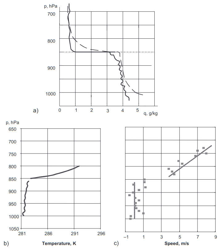
Humidity (a), temperature (b) and wind speed (c). All parameters experience sharp variations at the upper boundary of the atmospheric boundary layer
Studies of the energy spectrum of the turbulent fluctuations of the meteorological parameters (temperature, humidity, pressure and wind speed) have shown that the energy spectrum reveals three distinct regions:
- Large scale quasi-two-dimensional fluctuations in a range of frequencies from 10–6–10–4 Hz, the meso-meteorological minimum with low intensity of the fluctuations in the range 10–3–10–4 Hz and;
- A small scale three-dimensional fluctuation region with frequencies above 10–3 Hz.
Figure 2 shows the energy spectrum of fluctuations of the horizontal component of the wind speed in the atmosphere, where the ordinate corresponds to the product of the spectrum density S(ω) and the cyclic frequency ω of the variations in one of the meteorological components, and the abscissa corresponds to the frequency ω = 2π/T, T being a period of variations.
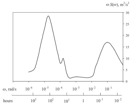
As observed in Figure 2, there are two major extremes of the function ω · S(ω) the high frequency maximum corresponds to a linear scale of turbulence of the order of tens and hundreds of meters, the low frequency maximum has a time scale of 5–10 days which is caused by synoptic variations (cyclones and anti-cyclones), the respective horizontal scale is thousands of kilometres and the vertical scale is of the order of 10 km. There is also an extended minimum in the spectrum ω · S(ω) that corresponds to the fluctuations with respective horizontal scales from 1 to 500 km and is called the meso-pause. The region of low frequency variation is called the macrorange while the region to the left of the meso-pause (high frequency variations) is called the micro-range.
The nature of the atmospheric turbulence is different in these two regions: in the macro-range the synoptic processes can be regarded as two-dimensional variations, while in the micro-range, with scales up to a hundred meters, the turbulence is three-dimensional and locally uniform. The mezo-pause is a transition region where a combined mechanism is observed. It is important to notice that by describing small-scale three-dimensional fluctuations in the micro-range region one can use Taylor’s hypothesis of “frozen turbulence” which allows a transformation from time to space-fluctuation scales by means of:
where:
- L is the spatial scale of the irregularities;
- f is the frequency of time variations in the refractive index, and;
- v is the mean speed of the incident flow.
It is then convenient to represent the dielectric permittivity in the form:
where:
In radio-meteorology mean characteristics of the meteoparameters are usually understood to be the values obtained by averaging over a 30 min interval, i. e. averaging is performed over a frequency interval the lower limit of which is positioned within the limits of the meso-meteorological minimum.
Standard Model of the Troposphere
Such conditions of refractivity constitute a model of standard linear atmosphere defined as:
and are applicable for heights less than 2 km. Let us consider this model in detail involving a geometrical optic presentation for wave propagation. Let us define “ray” as a normal to a wavefront propagating through the medium with varying refractivity n(z). As is known, the ray bends in such a medium and the bending is defined by Snell’s law.
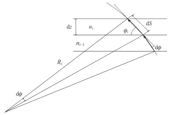
Introducing the horizontally stratified medium in terms of the set of thin layers with value of refractivity ni, i = 0, 1, …, such as illustrated in Figure 3, Snell’s law can be written as:
where ϕi is a sliding angle. Introducing the differentials of the ray direction dz, dS in the ith layer and differentiating both sides of Eq. (3) with respect to S:
Substituting dS = -dz/sin ɸi, we obtain:
The radius of curvature at any point, Ri = dS/dϕi, and using Eq. (5) it results that:
For the standard atmosphere with dn/dz = 39×10–6 km–1, the radius of curvature is given by:
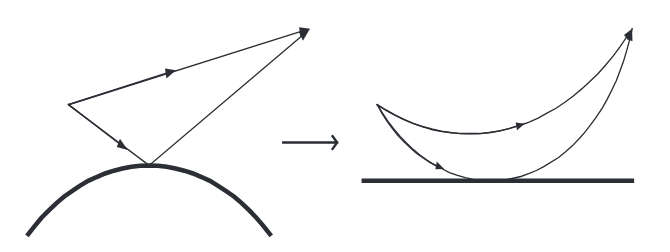
If the launch angle ɸi is close to the horizontal, the ratio ni/cos ɸi ≈ 1 and a propagation path can be described as a circle of radius R = 25 000 km, Figure 4(a). By comparison, the radius of the earth’s curvature is α = 6 370 km, and 1/α = 157×10–6 km–1. When the curvatures of both the propagation path and the earth are reduced by 39×10–6, as in Figure 4(b), the propagation path has an effective curvature of zero (which is a straight line) and that hypothetical earth has an effective curvature of (157-39)×10–6 km–1 = 118×10–6 km–1.
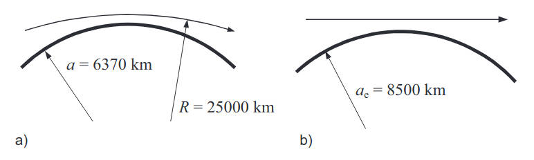
a) Ray refraction in a “normal” atmosphere with “true” earth radius α = 6 370 km. b) Effective ray refraction in case when the difference in curvatures of both ray and earth surface in (a) is compensated by introduction of the modified earth radius αe = 8 500 km
The equivalent radius of the sphere αe can therefore be defined as:
approximately, αe = 4/3α.
The modified refractive index can be defined as follows:
It is apparent that the second term in Eq. (9) is a compensation for the earth’s curvature. The modified refractivity M(z) is then given by:
As observed from Eq. (10) for the case of standard refraction, when γN = dN/dz = -39 N-units km-1, γM = dM/dz = 118 N-units km-1. As explained in Understanding Parabolic Approximation in Wave Propagation: Analytical Methods and Applications“Analytical Methods in the Problems of Wave Propagation in a Stratified and Random Medium”, modified refractivity comes logically from the parabolic approximation to the wave equations and effectively results in the introduction of the flat earth and additional curvature of the “rays” associated with radio waves propagating at low-angles along the earth’s surface, as shown schematically in Figure 5.
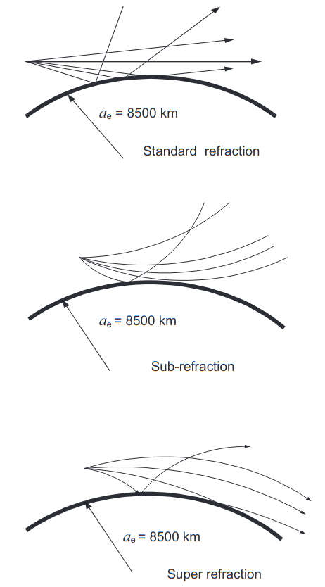
This traditional linear model of the troposphere provides some means of classification of the propagation mechanisms based on the value of the gradient of the refractivity in the lower troposphere, both conventional γN = dN/dz and modified refractivity γM = dM/dz. A very broad classification is concerned with the separation of the propagation into two classes: standard and non-standard. Figure 6 represents schematically the ray traces for three basic sub-classes of standard mechanisms of propagation in the troposphere:
- Standard refraction, when the vertical gradient of refractivity is very close to
- Sub-refraction, when γN > –39 N-units km–1, γM > 118 N-units km–1.
- Super-refraction, when γN < –39 N-units km–1, γM < 118 N-units km–1.
As seen from Figure 6 the sub-refraction and super-refraction are associated with bending the waves outwards and inwards to the earth’s surface respectively.
Non-standard mechanisms of radio wave propagation are related to some anomalies in the vertical distribution of the refractive index, namely the gradients cM become negative. These anomalies are in turn caused by some extremes in the vertical profiles of either the humidity or temperature.
Under such conditions the waves can be trapped inside a localised region associated with such negative gradients of modified refractivity, this effect is called “ducting” and the radio wave propagation mechanism is somewhat similar to propagation in a waveguide.
Non-standard Mechanisms of Propagation
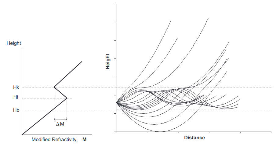
The term M-inversion is used to characterize the area of negative gradients of the M-profile, where dM/dz < 0. When M-inversions exist over some height interval, a radio-waveguide can be formed. The upper boundary of the waveguide is the height H at which dM/dz = 0, while the lower boundary zmin is given by M(zmin) = M(H), see Figure 9 later. The waveguide is elevated if zmin > 0. If zmin = 0 or the equation M(zmin) = M(H) has no solution, then the waveguide is classified as a surface wave-guide, Figure 7.
Most often M-inversions are formed in the lower and upper regions of the atmospheric boundary layer because of the local interaction between the turbulent air mass and either the surface or the free atmosphere above the ABL.
Evaporation Duct
One of the most important types of radio waveguide is the evaporation duct above the water surface which has a nearly permanent presence in the subtropical regions of the Pacific Ocean. It is formed as a result of the air in contact with the sea surface becoming saturated by water vapor at the surface temperature.
The water vapor content decreases logarithmically with height and the resulting M-profile has the form:
where:
- zr is the roughness parameter of the sea surface and;
- α = 106/α = 0,157 m–1 and α = 6 370 km, the earth’s radius.
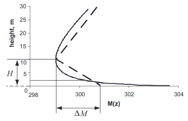
The M-profile (11) is can be constructed from the data of a standard hydrometeorological measurement. It describes quite well the height dependence of the M-profile under stable and neutral conditions of stratification in turbulence. The studies performed show that the thickness of the duct (inversion height H) is a function of the stability parameter of the turbulence at the water level layer and is functionally related to the inversion depth ΔM = M(zr) – M(H), Figure 7.
It should be noted that no analytical solution to the wave equation exists for the M-profile in form (11). While a numerical solution can be adopted with some modifications to Eq. (11), in some applications it might be preferable to replace Eq. (11) by a profile for which the analytical solution to a wave equation is known.
In particular, a common approach is to use a piecewise linear M-profile given by:
Comparison of the results obtained with both the piecewise linear approximation and the continuous M-profile (12) is presented in UHF Propagation in an Evaporation Duct“Some Results of Propagation Measurements and Comparison with Theory”. It has shown a satisfactory agreement of the results of calculations for the lower order modes. In fact, the discrepancies observed for the high order modes in terms of their propagation constants and therefore the height functions are not really important because those modes are significant in the transition area between the shadow and LOS regions, where, in turn, the mode presentation is hard to utilise because of the very slow convergence of the modal series. On the other hand, it was observed that the errors introduced by replacement of the continuous profile by a piecewise approximation for the lower modes do not exceed the errors produced by uncertainties in determining the values of the refractive index from data of standard hydro-meteorological measurements. The overall conclusion therefore is that the approximation (12) is a valid practical approach to analytically evaluate the propagation mechanism in the evaporation duct. In computer based prediction systems, where input radio-meteorological information can be collected in nearly real-time with substantial precision, the hydro-dynamical model of the evaporation duct Eq. (11) can be easily implemented. The common problem of calculating the propagation constants of the trapped (or significant) modes can be reduced to pre-calculated look-up tables and interpolation.
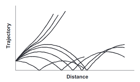
Figure 8 shows a schematic ray bending in the evaporation duct, which allows over-the-horizon radio wave propagation.
Elevated M-inversion
The most frequent cause of abnormally high signal level far beyond the horizon (200–500 km) is associated with the presence of elevated M-inversions. Those are formed in the subtropical region above the ocean as a result of powerful motion downwards in the center of an anticyclone and are usually called depression layers. The elevated M-inversions, also called elevated waveguides or inversion layers, are characterized by lower height of inversion Hi, the thickness of the layer with negative M-profile (M-inversion) ΔH = Hu-Hi and the depth of inversion, the so-called M-deficit ΔMi = M(Hi)-M(Hu), as shown in Figure 9.
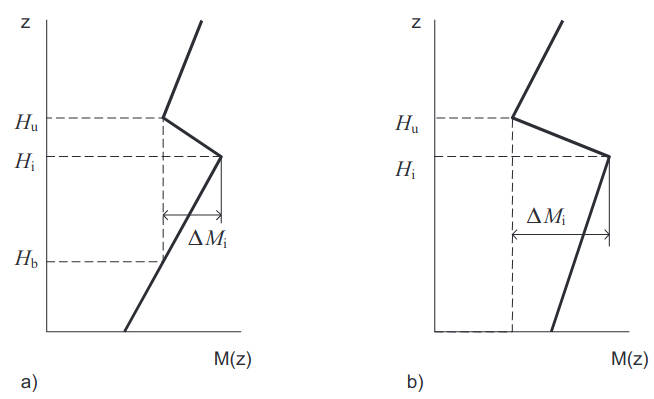
a) Elevated tropospheric duct in the height interval Hu > z > Hb; b) Surface based tropospheric duct in the height interval Hu > z > 0
Figure 10 shows schematic ray trajectories in an elevated duct when the source is placed inside its boundaries.
The observations indicate that characteristic values for the depression layers are as follows: Hi ≈ 200-1 500 m, ΔH ≈ 100-300 m, and ΔMi ≈ 10-30 units. The depression layers are normally observed as stable atmospheric formations existing over a wide area of the ocean surface. The height of inversion usually coincides with the height of the atmospheric boundary layer. The elevated M-inversion normally separates a convective boundary layer from the free atmosphere above, and in the direct vicinity of M-inversion turbulence alternates with laminar flow. Due to a penetration of convective elements from the lower atmospheric boundary layer the local temperature and gradients of the wind speed increase and as a result Kelvin–Helm-holtz waves develop. When these waves collapse they generate an intense turbulent structure.
Characteristic scales of the turbulent inhomogeneities in the depression layer can be estimated as follows: horizontal scale L||~500–1 000 m, vertical scale Lz ~100 m.
There is another important type of elevated M-inversion which is often formed in coastal regions due to the formation of a surface duct as a result of heating of the sea surface at sunrise and elevation of the surface M-inversion at night time. The elevated M-inversion is then unstable due to a developed convection.
Random Component of Dielectric Permittivity
The reverse transform is given by:
then:
Locally Uniform Fluctuations
The important advantage of using a structure function is that it makes sense even when the correlation function does not exist, Bε(0) → ∞. However, if it does exist then the following relationship is valid:
When Bε(∞) → 0, Dε(∞) → 2Bε(0) and:
The structure function Dε is related to a spatial spectrum Φε via the relationships:
As observed from Eq. (30) the structure function Dε(ρ) is unlimited by a scale of fluctuations and allows the existence of turbulent bursts of any scale, which is contradictory to the applicability of the Kolmogorov–Obukhov model which is itself limited to an inertial interval of the locally isotropic turbulence.
In order to limit the external scales of the fluctuations to an inertial interval of the turbulence and to make the model consistent one can introduce a maximum scale L0 of the turbulent fluctuations and therefore a “saturation” feature in the behavior of the structure function:
A combined structure function for locally uniform and isotropic fluctuation in δε can be written as follows:
The applicability of Kolmogorov’s model (34) for the atmospheric boundary layer over the ocean surface has been studied in Ref. The basic observations are as follows:
- A one-dimensional spectrum of the turbulent fluctuations in the horizontal plane follows Kolmogorov’s model up to scales: L|| ~10-100 m. The spectrum interval over which the postulates of a locally isotropic turbulence are valid depends on the stability of the atmosphere and decreases greatly when the stability intensifies. In the case of very stable stratification associated with the presence of M-inversions the turbulent structure reveals significant anisotropy of the large-scale fluctuations.
- At heights above the surface comparable with the heights of the swells, the state of the sea surface reveals a significant impact on a form of the spectrum of turbulent fluctuations. This manifest itself in the form of flares in spectral density at the frequencies corresponding to the energy-bearing frequencies of the sea waves. The amplitude of the wave perturbations decreases with height and has no practical effect on the form of the spectrum at heights of 15-20 m above the surface.
- The intensity of the high-frequency turbulent fluctuations depends parametrically on the height above the surface. In a low-frequency domain (the buoyancy and energy intervals) one must include additional parameters in the model of spectrum: the thickness of the atmospheric boundary layer and some parameters characterizing the roughness of the sea surface.
It can be stated that despite numerous studies, a physically justifiable model for a three-dimensional spectrum of fluctuations in the index of refraction within the atmospheric boundary layer does not yet exist. The anisotropy of the spatial fluctuations in the refractive index is commonly introduced via the anisotropy parameter α = Lz/L|| in the following model of the spectrum:
where Cε⟂ and Cεz are structure constants in the horizontal plane and over height respectively, as observed they are not independent and are related via:
The observations suggest that the value of the anisotropy parameter α itself is a function of the external scale of the turbulent fluctuations and can be estimated to be of the order of α ~0,1-0,2 for Lz ~1 m at the heights close to the water level. At the upper boundary of ABL the parameter a may vary from a ~0,8 for L|| ~15 m to α ~0,005 for L|| ~10 000 m.

- Jensen, N.O., Lenshow, D.H. An observational investigation on penetrative convection. J.Atmos.Sci., 1978, 35(10), 1924–1933.;
- Monin, A.S., Yaglom, A.M. Statistical Fluid Mechanics, Vol.1, MIT Press, Cambridge, MA, 1971, p. 769.;
- Gossard, E.E. Clear weather meteorological effects on propagations at frequencies above 1 GHz, Radio Sci., 1981,16(5), 589–608.;
- Tatarskii, V.I. The Effects of Turbulent Atmo- sphere on Wave Propagation, IPST, Jerusalem, 1971.;
- Gavrilov, A.S., Ponomareva, S.M. Turbulence Structure in the Ground Level Layer of the Atmosphere. Collected Data, Meteorology Series, No.1, Research Institute for Meteorological Information, Obninsk (in Russian), 1984.;
- Kukushkin, A.V., Freilikher, V.D. and Fuks, I.M. Over-the-horizon propagation of UHF radio waves above the sea , Radiophys. Quantum Electron. (translated from Russian), Consultant Bureau, New York , RPQEAC 30 (7), 1987, 597–620.;