Exploring UHF Propagation in Evaporation Ducts

Discover the dynamics of UHF propagation in evaporation ducts in this detailed article. We present key measurement results, theoretical comparisons, and insights into perturbation theory for normal waves in a stratified troposphere. Topics include problem formulation, linear and smooth distortion, height functions, and the effects of linear-logarithmic profiles near the sea surface.

СодержаниеСвернуть

Some Results of Propagation Measurements and Comparison with Theory
Perturbation Theory for the Spectrum of Normal Waves in a Stratified Troposphere
Problem Formulation
Linear Distortion
Smooth Distortion
Height Function
Linear-Logarithmic Profile at Heights Close to the Sea Surface

The most important characteristic of the troposphere in terms of radio wave propagation is a refractivity profile averaged over the coordinates tangential to the sea surface, i. e., an M-profile in a “stratified” troposphere:

M (z) = 10^{6} [\frac{ε (z) - 1}{2} + \frac{z}{a}] = 10^{6} [\frac{ε (z) - 1}{2}] + 0, 157 z

where z is the height above the sea surface, the gradient 0,157 N-units m^–1 takes into account the curvature of the earth in the case of normal refraction. According to radio-meteorological and refractometer world-wide data, the gradient of the modified refractivity g_m = dM/dz is less than the critical gradient g_c = –0,157 N-units m^–1 for more than 50 % of the time of observation over the sea surface. In those conditions the surface M-inversion forms an evaporation duct, which signifi- cantly affects the process of radio wave propagation by trapping the waves radiated in a selective frequency band.

The simplest characteristic of the ducting properties of the surface based M-inversion is the “critical” wavelength λ_c defined as:

λ_{c} = \frac{4}{3} 10^{- 3} β Z_{s} \sqrt{2 (M (0) - M (Z_{s}))}, m E q . 1

and:

β = \int_{0}^{1} \sqrt{q (ς) d ς} .

Parameter ς is introduced in Ref. as ς = z/Z_s thus providing a meaningful definition for:

q (\frac{z}{Z_{s}}) = 4 \frac{M (z) - M (Z_{s})}{M (0) - M (Z_{s})}

with q(0) = 4, q(1) = 0.

Frequently observed surface M-inversions of height up to 15 m are capable of ducting radiowaves in a cm band with wavelength λ ≤ λ_c ~ 5 cm. With increasing wavelength the impact of the evaporation duct is weakened, though the attenuation of the waves with wavelength λ > λ_c may still be significantly less than in the case of normal refraction. Fock showed that the attenuation of the field in the shadow region follows the exponential law exp (-γx), where x is the distance from the horizon, and the magnitude of the attenuation exponent γ depends on the curvature of the M-profile at the minimum point at z = Z_s:

γ \infty 2 π 10^{- 3} \frac{Z_{s} M^{''} (z = Z_{s})}{β \sqrt{2 ∆ M}} Θ E q . 2

where Θ is a coefficient determined by the imaginary part of the propagation con- stantt_n.

The above estimates are qualitative in nature. To calculate the field we need to solve the boundary problem (26), (27).

In a stratified troposphere, calculation of the electromagnetic field beyond the horizon is truncated to the determination of the complex propagation constants E_n and the height-gain functions χ_n(z) of the normal waves. The total field is then composed of a superposition of the normal waves, which converge in a shadow region. The analytical solution to the problem is known only for a few etalon problems with a limited number of selected M-profiles. In the general case the modal formalism will require a numerical solution of the characteristic equation for propagation constants and, in many cases, numerical integration of the differential equations for the height-gain functions.

This article is arranged as follows: First in Section “Some Results of Propagation Measurements and Comparison with Theory”, we discuss some results of the propagation measurements and comparison with the prediction based on existing propagation models in order to highlight the current status of the theory and the remaining problems in modelling the propagation phenomena. Then we introduce the perturbation theory for the normal waves and propagation constants in Section “Perturbation Theory for the Spectrum of Normal Waves in a Stratified Troposphere”. The perturbation theory provides a means of analytic study of the spectrum of the propagation constants and the height-gain functions with small variations of the M-profile from the etalon profile for which the solution is known.

Spectrum of Normal Waves in an Evaporation Duct“Detailed Wave Spectrum Analysis in Evaporation Ducts” is dedicated to the determination of the spectrum of normal waves in an evaporation duct. The solution is limited to the case of a stratified troposphere that is commonly used in existing radio coverage prediction systems.

In Coherence Function in a Random and Non-uniform Atmosphere“Understanding Coherence Function in Random Atmospheres” we will study the impact of random fluctuations in refractive index on propagation inside an evaporation duct. The results suggest that the impact may be significant in the frequency range 10 GHz and above.

Excitation of Waves in a Continuous Spectrum and Evaporation Duct with Two Trapped Modes“Wave Excitation in Inhomogeneous Evaporation Ducts” deals with the height gain structure of the field inside and outside the evaporation duct for the case of scattering on the turbulent fluctuations in the refractive index. It is shown that scattering on random inhomegeneities of the refractive index leads to a smoother height dependence of the field beyond the horizon compared with duct theory. The results seem to be closer to observations.

Some Results of Propagation Measurements and Comparison with Theory

Systematic studies of radiowave propagation over the sea surface started in the 1940s, driven by the development of radar, and are still underway due both to the importance of the problem and advances in technology and applications. Several comprehensive programs of radio-meteorological measurements performed in the 1940s and 1950s still provide a benchmark reference for further studies due to the exceptionally high quality of the obtained results.

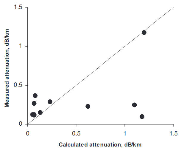
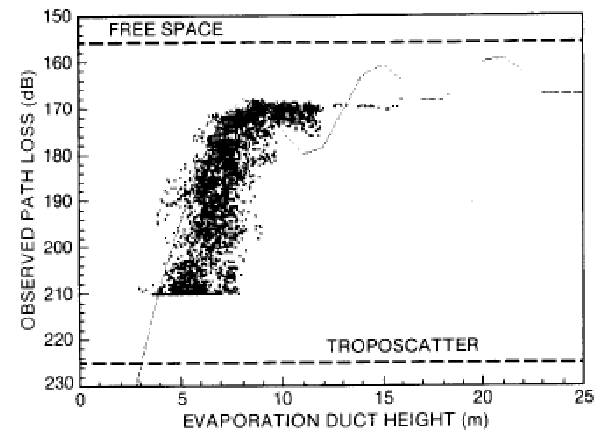
Here we briefly review the major results. The propagation measurements were performed at two frequencies 3 GHz and 10 GHz over a sea path extending to several hundred kilometres and were supported by shipboard meteorological measurements of the temperature, water vapor and air pressure. The restored M-profile was then averaged over several measurements along the propagation path and that averaged profile was approximated by a linear-exponential M-profile (Peceris’s model) in order to perform a theoretical calculation of the propagation loss and to estimate the attenuation rate of the signal beyond the horizon. A sample of the comparison of the experimental attenuation rates with Peceris’s duct model is presented in Figure 1 for 3 and 10 GHz measurements.

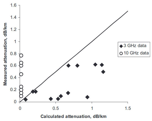
Peceris duct model — Fig. 1 Comparison of the measured and modelled attenuation rates at 3 and 10 GHz

As observed from Figure 1, the measured attenuation rates of the 3 GHz signal tend persistently to be less than predicted from the linear-exponential model of an evaporation duct. In contrast, the measured attenuation rate significantly exceeded the theoretical estimates. The conclusion drawn in 1949 was that there was a significant quantitative discrepancy between the theory and the measurements.

A second revision of the reference data was performed in the 80s. A new advanced computer-based model of an evaporation duct was implemented to calculate the propagation constants and height gain functions. For comparison of the theory and measurements it was decided to limit to the distances to less than 150 km. The analysis of the measured data led to the conclusion that the evaporation ducts restored at the time of measurement may explain the behavior of the signal in that sub-range, while at larger distances the observed signal levels might be explained by either single-scattering theory in the case of low level signals or the presence of the elevated M-inversion. The last was difficult to analyse since there were no adequate radiosound measurements performed at the time of the radio measurements.

Figure 2 shows the result of a comparison of the same measured data as for Figure 1 at 3 GHz with a computer-based calculation for bilinear approximation of the averaged M-profile. As observed, the measured attenuation rates are still less than those predicted from the evaporation duct model. Major discrepancies are observed for lower duct heights, in conditions of unstable stratification.

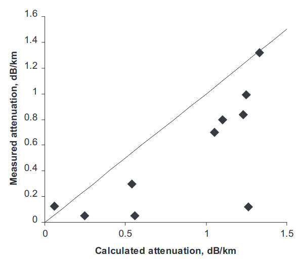
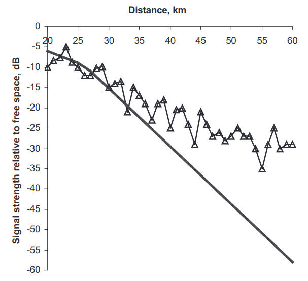
Calculation for bilinear approximation — Fig. 2 Comparison of the measured and modelled attenuation rates at a frequency of 3 GHz. The evaporation duct is modelled by a bilinear M-profile

One of the measured samples is shown in Figure 3, where the restored M-profile reveals an evaporation duct with parameters: Z_s = 6 m, and ΔM = 2 N-units. Such discrepancy tends to be persistent in other measurements and cannot just be explained by unavoidable errors in measurements of the meteorological data.

Fig. 3 Comparison of the measured and predicted signal levels at 3 GHz in the presence of an evaporation duct with height 6 m and M-deficit of 2 N-units

In principle, the bilinear model tends to underestimate the attenuation rate compared with the more realistic linear-logarithmic model of the evaporation duct. This leads to the conclusion that the other models of propagation may provide a somewhat intermediate situation when the evaporation duct is not sufficiently strong to support the trapping mechanism by itself, however, negative gradients of the refractivity provide significant enhancement of the propagation beyond the horizon. One of the unusual but possible mechanisms is studied in Scattering Mechanism of Over-horizon UHF Propagation“Scattering Mechanism of Over-Horizon UHF Propagation”.

It should be also noted that, in the presence of a strong evaporation duct with heights exceeding 10 m, the waveguide mechanism is more pronounced at a frequency of 3 GHz, and comparison of the evaporation duct model with measurements is rather satisfactory. A typical example is shown in Figure 4 for an evaporation duct with height Z_s = 14 m, and ΔM = 7 N-units. The heights of the transmitting and receiving antennas are 18 m and 6 m, respectively.

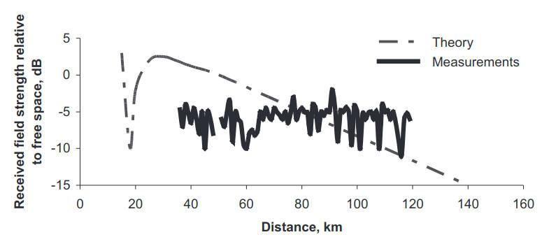
Figure 5 shows the comparison of the revised attenuation rates for frequency 10 GHz. As observed, the spread of the data points relative to the bisector is wider than in Figure 2 for the 3 GHz data.

In most cases the measured attenuation rates are higher than predicted and sometimes the actual propagation mechanism can be questioned, for example in Figure 6. In general, the evaporation ducts with a height of over 10 m are supposed to provide a waveguide mechanism at 10 GHz with attenuation rate of several hundredth dB km^–1 (chiefly due to a finite impedance of the sea surface). On the other hand, the attenuation rates measured during the experiment were never less than 0,2 dB km^–1 at 10 GHz, even in the presence of a very strong and stable with distance evaporation duct.

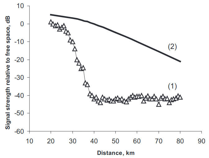
Graph - attenuation rates — Fig. 6 Comparison of the measured (1) and predicted (2) signal levels at 10 GHz in the presence of an evaporation duct with height 9 m and M-deficit of 3 N-units

Figure 7 shows the results obtained when the height of the receiving antennas was changed during the experiment. The evaporation duct structure was stable over the distance and the assumption of the uniformity of the duct in a horizontal plane was quite reasonable during the experiment. The evaporation duct with parameters Z_s = 14 m, and ΔM = 7 N-units forms two trapped modes at frequency 10 GHz.

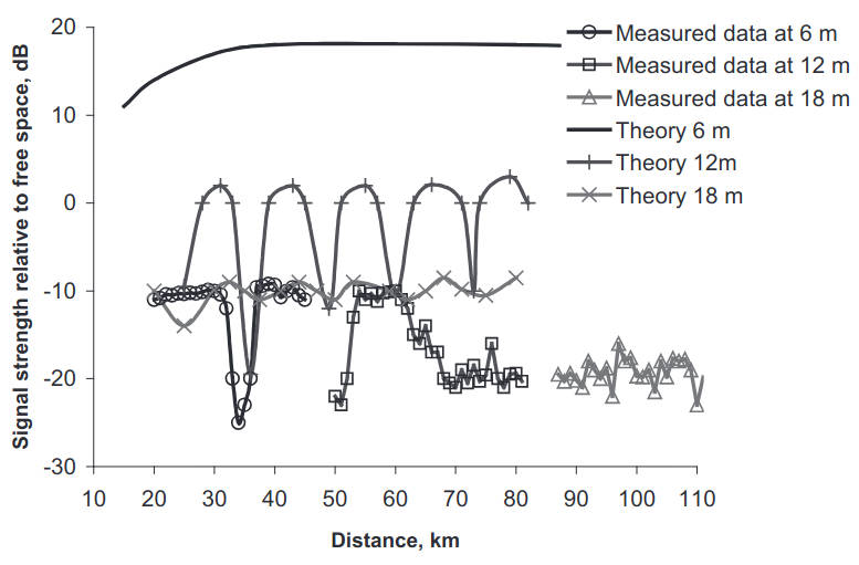
Presence of an evaporation duct — Fig. 7 Comparison of measured and predicted data at 10 GHz in the presence of an evaporation duct with height 14 m and M-deficit of 7 N-units. The transmitting antenna is mounted at a height of 6 m

The interference between these modes is responsible for the ripples in the theoretical curve for the received signal at a height of 12 m. At a height of 6 m the interference is not pronounced since the second mode has a minimum at this height. A receiver placed above the evaporation duct at a height of 18 m is supposed to receive the em field by penetration through a potential barrier, or, in other words, by a “leak” of the trapped modes. Theoretically predicted signal levels at 18 and 6 m should then differ by 20 dB, as shown in Figure 7. On the other hand, the measured data do not reveal any significant difference with the height of the receiving antenna. This situation is not unique and is observed in other experiments. One possible explanation of the above phenomena is provided in Excitation of Waves in a Continuous Spectrum and Evaporation Duct with Two Trapped Modes“Wave Excitation in Inhomogeneous Evaporation Ducts”.

We may conclude that significant development in modelling the evaporation duct structure in the lower part of the marine boundary layer resulted in the availability of computer-based tools capable of reasonably good prediction of the shipboard radar coverage in nearly real time over a wide range of frequency bands from VHF to EHF.

The statistical assessment of the evaporation duct contribution also demonstrates unexpectedly high signal levels beyond the horizon in the case of weak ducting conditions at frequencies 0,6 GHz and 3 GHz, where the evaporation ducts with heights less than 10 m are too weak to ensure a single trapped mode. Nonetheless, the received signal tends to be higher than predicted, as shown in Figure 8.

Evaporation duct and path-loss — Figure 8 Path-loss versus evaporation duct height for the North Sea experiment

It was suggested that the observed high level signals might be caused by propagation mechanisms other than an evaporation duct. One of the conclusions emphasised is that the height dependence of the received field is not as significant as may follow from the evaporation duct theory and, basically, high altitude antennas are preferable. In terms of the optimal frequency the results of the measurements suggest the 10–20 GHz band is an optimal band where the evaporation duct makes a strong impact without being counteracted by gaseous absorption at higher frequencies.

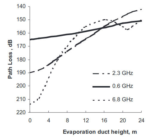
A clear demonstration of the advances in radar coverage prediction and range detection enhancement due to an evaporation duct for 18 GHz radar measurements. Similar results for propagation experiments in a range from 3 to 94 GHz. The predicted values of the path loss are depicted as a curve in Figure 9.

Path losses — Fig. 9 Observed path losses for evaporation duct conditions at 17,7 GHz

The ripples for the higher duct’s height are caused by the presence of several trapped modes and corresponding restructuring of the height gain function of the total trapped field in the waveguide. While overall agreement between prediction and measurements is very good the prediction tends to underestimate the path loss for lower duct heights. It might be noted that the scattering on the rough surface is modelled in a rather conservative way using the Kirchhoff approximation, which is applicable to a coherent field component. Nonetheless, an additional attenuation factor, like scattering at random fluctuations in the refractive index, might be taken into account for possible improvement in the prediction model. It may also be pointed out that the spread of the data points in Figure 9 tends to be more close and symmetrical relative to the prediction curve, which may again suggest the importance of the full treatment of the scattering mechanism. We recall these arguments later in Spectrum of Normal Waves in an Evaporation Duct“Detailed Wave Spectrum Analysis in Evaporation Ducts” where the scattering mechanism is described.

Another experiment in the millimetre wave range for 94 GHz propagation. The results obtained demonstrated the validity of the evaporation duct mechanism in this frequency band and gave good agreement between the measurements and the theory of the evaporation duct, with some underestimation of predicted path loss with an average value of error of 10 dB. It might be noted that while the prediction model has made use of the Kirchhoff theory of the scattering at a rough sea surface, the model did not take into account scattering on turbulent fluctuations in the refractive index.

Perturbation Theory for the Spectrum of Normal Waves in a Stratified Troposphere

The presence of stratified inhomogeneities of the refractive index results in a considerable change in the field structure in the region of geometric shadow. A complete solution to the problem of wave propagation in a stratified troposphere, in which the refractive index depends only on the height h above the earth’s surface, was obtained by Fock. He showed that for large values of the parameter m = (ka/2)^1/3 ≫ 1, here k is the wave number and a is the earth’s radius, the problem can be simplified by transition from a spherically stratified to a plane-stratified medium. Such a simplification is provided through the use of the Understanding Parabolic Approximation in Wave Propagation: Analytical Methods and Applicationsparabolic approximation and introduction of the modified permittivity:

ε_{m} (h) = ε + 2 \frac{h}{a} .

Even in this simplified formulation an analytical solution can be obtained only for a few standard problems with a limited set of permittivity profiles ε_m(h). In the general case the analysis of the propagation conditions comes down to a numerical solution for an eigenvalue problem with complex propagation constants. In several cases the function ε_m(h) differs little from the “etalon” function, as for instance in the case of weak refraction. Therefore, some need arises to construct a perturbation theory for “open” system for which the spectrum of eigenvalues (propagation constants is complex and eigenfunctions (height factors for the Wave Field Fluctuations in Random Media over a Boundary Interfacewave field χ_n(h)) grow exponentially with height, χ_n(h) → ∞, h → ∞. A similar problem arises in quantum mechanics with the study of the decay of quasi-stationary states. Perturbation theory for that case was developed by Zeldovitch, although the essential assumption was made on the finiteness of the potential (the analogue of ε_m(h)) at (h) → ∞. Such a condition is not satisfied in the problem of wave propagation in a stratified troposphere:

ε_{m} (h) \to 2 h / a as h \to \infty .

Here we describe a generalisation of the perturbation theory to the case of potentials unlimited at (h) → ∞.

Problem Formulation

The field attenuation factor V for a point source in the spherically stratified medium can be represented by superposition of normal waves:

V (x, γ, γ_{0}) = 2 {\sqrt{π x e}}^{j π 4} \sum_{n = 1}^{\infty} e^{j x t_{n}} \frac{χ (γ, t_{n}) χ (γ_{0}, t_{n}) χ^{*} (0, t_{n})}{\frac{\partial}{\partial t_{n}} χ (0, t_{n})} E q . 3

where we introduce dimensionless coordinates:

x = m D / a, γ = k h / m, k = k_{0} \sqrt{ε (h \to \infty)},

k₀ – is the wave number in a vacuum, and;
D – is the distance along the earth’s surface from the source of radiation.

The transmitter (point source) is situated at height h₀ and the receiver at height h, respectively. The height functions χ(γ, t_n) are governed by the equation:

\frac{d^{2}}{d γ^{2}} χ (γ, t_{n}) + [U (γ) - t_{n}] χ (γ, t_{n}) = 0 E q . 4

and satisfy the following boundary conditions:

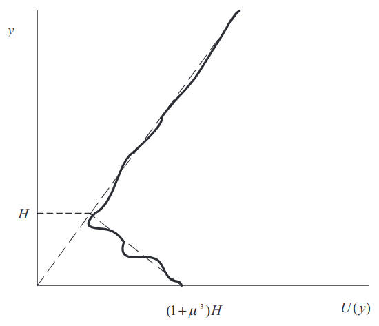
χ (0, t_{n}) = {0, \frac{δ}{d γ} \{a r g (χ (γ, t_{n}))\}}_{γ \to \infty} > 0 . E q . 5

Equations (4) and (5) determine a discrete spectrum of propagation constants t_n. We represent the modified refractive index U(γ) = m²(ε(γ)-1)+γ, as shown in Figure 10, in the form U(γ) = U₀(γ)+δU(γ), where U₀(γ) is the unperturbed index of refraction for which the solution to the boundary value problem Eqs. (4) and (5) is known. We shall treat δU(γ) as the perturbations to the etalon profile U₀(γ).

$Refractive index$

Figure 10 Refractivity profile with distortion

We introduce the logarithmic derivative:

z_{n} (γ) = \frac{d χ (γ, t_{n})}{d γ} \cdot χ^{- 1} (γ, t_{n}) E q . 6

through which the height function is expressed as:

χ (γ, t_{n}) = l i m_{σ \to 0} χ (σ, t_{n}) \cdot e x p (\int_{}^{γ} z_{n} (γ^{'}) d γ^{'}) . E q . 7

For z_n(γ) we can obtain the equation:

z_{n}^{'} (γ) + z_{n}^{2} (γ) + U_{0} (γ) + δ U (γ) - t_{n} = 0 . E q . 8

We seek z_n(γ) and t_n in the form:

z_{n} (γ) = z_{n}^{0} (γ) + δ z_{n} (γ); t_{n} = t_{n}^{0} + δ t_{n} E q . 9

where

z_{n}^{0} (γ)

and

t_{n}^{0}

correspond to the height function of the unperturbed Eq. (4) and δz_n ~ δt_n ~ δU. Substituting Eq. (9) into Eq. (8), we obtain the equation for correction to the height function:

δ z_{n}^{'} = - 2 z_{n}^{0} (γ) δ z_{n} (γ) + δ t_{n} - δ U (γ) . E q . 10

The solution to Eq. (10) has the form:

δ z_{n} (γ) = χ_{0}^{- 2} (γ, t_{n}^{0}) \int_{0}^{γ} χ_{0}^{2} (γ^{'}, t_{n}^{0}) [δ t_{n} - δ U (γ^{'})] d γ^{'} . E q . 11

It is reasonable to assume that perturbations δU(γ) to a standard profile can be neglected at sufficiently large heights, then the solution to Eq. (4) as γ → ∞ has the same form as that of the standard problem

χ_{0} (γ, t_{n}) :

{δ z_{n} (γ)}_{γ \to \infty} \approx δ [χ_{0}^{- 1} (γ, t_{n}^{0} + δ t_{n}) \frac{d}{d γ} χ_{0} (γ, t_{n}^{0} + δ t_{n})] = \frac{δ t_{n}}{χ_{0}^{2} (γ, t_{n}^{0})} \cdot [χ_{0} (γ, t_{n}^{0}) \frac{\partial^{2} χ_{0} (γ, t_{n}^{0})}{\partial γ \partial t_{n}} - \frac{\partial χ_{0} (γ, t_{n}^{0})}{\partial γ} \frac{\partial χ_{0} (γ, t_{n}^{0})}{\partial t_{n}}] . E q . 12

Substituting Eq. (12) into Eq. (11), we obtain the equation for correction to the propagation constant:

δ t_{n} = N^{- 1} {l i m}_{γ \to \infty} \int_{0}^{\infty} δ U (γ^{'}) χ_{n}^{2} (γ^{'}) d γ^{'} E q . 13

where:

χ_{n} (γ) \equiv χ_{0} (γ, t_{n}^{0}) .

Equation (13) differs from the usual equation of perturbation theory in two aspects:

first, there is a
$χ_{n}^{2} (γ)$
under the integration instead of the square of the absolute value |χ_n(γ)|² and;
second, instead of the norm, which does not exist in the present case, there is the finite term N equal to:

N = {l i m}_{γ \to \infty} \{\int_{0}^{γ} [χ_{n}^{2} (γ^{'}) - χ_{n} (γ^{'}) \frac{\partial^{2} χ_{n} (γ^{'})}{\partial \dot{γ} \partial t_{n}} + \frac{\partial χ_{n} (γ)}{\partial γ^{'}} \frac{\partial χ_{n} (γ)}{\partial t_{n}}] d γ^{'}\} = {(\frac{\partial χ_{n}}{\partial γ} \frac{\partial χ_{n}}{\partial t_{n}})}_{γ = 0} E q . 14

In the case of the troposphere the variation of the modified refractive index becomes linear at large enough heights and Eq. (14) takes the form:

N = {l i m}_{γ \to \infty} \{\int_{0}^{γ} [χ_{n}^{2} (γ^{'}) - w_{1}^{2} (t_{n}^{0} - γ^{'})] d γ^{'}\} - {[w_{1}^{'} (t_{n}^{0})]}^{2},

where

w_{1} (t_{n}^{0} - γ)

is an Airy function which is a solution to the standard problem (4) and (5) with U₀(γ) = γ.

In the case of normal refraction:

U_{0} (γ) = γ, χ_{n} (γ) = w_{1} (t_{n}^{0} - γ)

for all 0 < γ < ∞. The parameter a shall be understood as equivalent to the earth’s radius. The propagation constants in this case are determined from the solution to a transcendent equation

w_{1} (t_{n}^{0}) = 0

and for large numbers n they have an asymptotic form:

t_{n}^{0} = τ_{n} e^{j \frac{π}{3}}, τ_{n} = {[3 / 2 (n - 1 / 4) π]}^{2 / 3} .

Equation (14) is then reduced to:

N = {l i m}_{γ \to \infty} \{\int_{0}^{γ} w_{1}^{2} (t_{n}^{0} - γ^{'}) d γ^{'} + (t_{n}^{0} - γ) w_{1}^{2} (t_{n}^{0} - γ) - {[w_{1}^{'} (t_{n}^{0} - γ)]}^{2}\} . E q . 15

Calculating the integral appearing in Eq. (15):

\int w_{1}^{2} (- x) d x = x w_{1}^{2} (- x) + {[w_{1}^{'} (- x)]}^{2} E q . 16

and using the boundary condition (5), we obtain:

N = - {[w_{1}^{'} (t_{n}^{0})]}^{2}

δ t_{n} = - {[w_{1}^{'} (t_{n}^{0})]}^{- 2} \int_{0}^{\infty} δ U (γ) w_{1}^{2} (t_{n}^{0} - γ) d γ . E q . 17

Equation (17) allows one to find explicitly the correction terms δt_n to the complex propagation constants

t_{n}^{0}

of the normal wave for arbitrary distortion δU(γ) of the linear profile of the refractive index. Of course the limitation is that the correction terms prove to be small, i. e.

|δ t_{n}| ≪ |t_{n}^{0} - t_{n - 1}^{0}| .

It should be noted that in the case of large perturbation δU(γ) a new branch of the spectrum of the normal modes could arise, that case is outside the scope of the problem considered here.

Linear Distortion

Let us consider a linear distortion:

δ U (γ) = \{\begin{cases} (1 + μ^{3}) (H - γ), γ \leq H \\ 0, γ > H \end{cases}) E q . 18

where 1+μ³ is the gradient of the modified refractive index in the height range 0 < γ ≤ H as shown in Figure 10. The equation for the spectrum t_n of the normal modes was Basics of Fock’s Theory – the Hartree-Fock Approach to Evaporation Ductsderived by Fock, its solution cannot be obtained analytically and requires application of numerical methods. Application of perturbation theory in form (17) allows investigation of the t_n-spectrum in a considerably simple way.

Let the height of distortion be small, assuming that H ≪ τ_n and τ_n ≫ 1. Then the phase of the argument of the Airy function lies within the sector (π/3, 2π/3) and the asymptotic form of

w_{1} (t_{n}^{0} - γ)

is as follows:

w_{1} (t_{n}^{0} - γ) ~ {(t_{n}^{0} - γ)}^{- 1 / 4} \{e^{\frac{2}{3} {(t_{n}^{0} - γ)}^{3 / 2}} + j e^{- \frac{2}{3} {(t_{n}^{0} - γ)}^{3 / 2}}\} . E q . 19

Substitute Eqs. (18) and (19) into Eq. (17) and expand the exponentials in Eq. (19) in a series in powers of

γ / t_{n}^{0} .

Retaining the linear terms, which is valid when inequality

H^{2} ≪ \sqrt{τ_{n}}

holds, we obtain:

δ t_{n} = j (1 + μ^{3}) {(t_{n}^{0})}^{- 1 / 2} {[w_{1}^{'} (t_{n}^{0})]}^{- 2} \{2 - e^{- 2 H \sqrt{t_{n}^{0}}} + e^{2 H \sqrt{t_{n}^{0}}}\} . E q . 20

When the stronger inequality H² τ_n ≪ 1 applies we can obtain from Eq. (20):

δ t_{n} = - (1 + μ^{3}) \{\frac{H^{4}}{12} + \frac{H^{5} t_{n}^{0}}{90}\} . E q . 21

As observed from Eq. (21), increase in the height H or depth (1+μ³)H of inversion in the refractive index leads to a decrease in the real and imaginary components of the propagation constant t_n, that corresponds to an increase in the phase velocity of the normal wave and a decrease in its attenuation.

The applicability of the perturbation theory is limited by a small variation to the propagation constant:

|δ t_{n}| ≪ |t_{n}^{0} - t_{n - 1}^{0}| \approx \frac{π}{\sqrt{τ_{n}}} . E q . 22

Inequality (22) in conjunction with H²τ_n ≪ 1 yields the limits of applicability of Eq. (21):

H ≪ m i n [τ_{n}^{- 1 / 2}, {(\frac{12}{(1 + μ^{3})})}^{1 / 4} τ_{n}^{- 1 / 8}] E q . 23

and, for Eq. (20):

H ≪ \frac{1}{\sqrt{τ_{n}}} \ln (\frac{16 τ_{n}^{3 / 2}}{1 + μ^{3}}) . E q . 24

Let us consider another limiting case, when the height of distortion is large H ≫ τ_n. We represent the integral in Eq. (17) as the sum of integrals over the arc of radius H in the sector of angles (0, π/3) and over the ray arg γ = π/3:

\int_{0}^{H} (H - γ) w_{1}^{2} (t_{n}^{0} - γ) d γ = I_{1} + I_{2},

I_{1} = \int_{0}^{H e^{j π / 3}} (H - γ) w_{1}^{2} (t_{n}^{0} - γ) d γ,

I_{2} = j H \int_{0}^{π / 3} (1 - e^{j φ}) w_{1}^{2} (t_{n}^{0} - H e^{j φ}) d φ .

In the integral I₁ we make a change in the variable γ = τe^jπ/3 and use the property of the Airy function w₁(xe^jπ/3) = 2e^jπ/3 ν(-x):

I_{1} = 4 e^{j 2 π / 3} \int_{0}^{H} (H - τ e^{j π / 3}) ν^{2} (τ - τ_{n}) d γ . E q . 25

The upper limit of integration in Eq. (25) can be extended to infinity since the Airy function ν(τ-τ_n) decreases exponentially for τ > τ_n. Then, using Eq. (16) we obtain:

I_{1} \approx 4 e^{j 2 π / 3} H \int_{0}^{\infty} ν^{2} (τ - τ_{n}) d γ = - 4 e^{j 2 π / 3} H \sqrt{τ_{n}} . E q . 26

To estimate integral I₂ we use the asymptotic behavior of the function

w_{1} (t_{n}^{0} - γ)

for large negative arguments:

where:

Ψ (φ) = 4 / 3 H^{3 / 2} e^{j 3 ϕ / 2} - 2 \sqrt{H} e^{j ϕ / 2} t_{n}^{0} .

The main contribution to the integral (27) comes from the region of small φ where the only linear terms can be retained in the expansion of the integrand. Then we obtain:

I_{2} ≅ \frac{1}{4 H^{3 / 2}} e x p (j \frac{4}{3} H^{3 / 2} - 2 j \sqrt{H} t_{n}^{0} + j \frac{π}{2}) . E q . 28

Substituting Eqs. (28) and (26) into Eq. (17) we obtain:

δ t_{n} = (1 + μ^{3}) H [1 - \frac{j}{16 τ_{n} H^{5 / 2}} e x p (j \frac{4}{3} H^{3 / 2} - 2 j \sqrt{H} t_{n}^{0})] . E q . 29

As observed from Eqs. (29) and (21), the correction factor dtn grows exponentially with number n since the imaginary part of the propagation constant is Im t_n~n^3/2, and hence the inequality (22) ceases to be satisfied, starting with certain n. It can be shown, however, that this result is a consequence of the “non-physical” nature of the broken linear profile. For smooth functions U(γ) that actually describe realistic behavior of the refraction index, the dt_n-dependence on a wave-number n has a fundamentally different character (see, for instance, Eq. (40) below).

In fact, performing integration by parts in Eq. (17), we can write:

δ t_{n} = - N^{- 1} \int_{0}^{\infty} \frac{d δ U (γ)}{d γ} F_{n} (γ) d γ E q . 30

where:

F_{n} (γ) = \int_{0}^{γ} w_{1}^{2} (t_{n}^{0} - γ^{'}) d γ^{'}

behaves as

1 / 2 t_{n}^{0} e x p (2 t_{n}^{0} \sqrt{γ})

for large numbers n:

\sqrt{τ_{n}} γ ≫ 1 .

If δU(γ) is a function continuous along y altogether with its derivatives and which decreases sufficiently at infinity, then integration in Eq. (30) will result in values of δt_n which decrease for large n.

In the case where δU(γ) is abruptly reduced to zero at γ = H (a discontinuity of the first kind), a singularity of a delta-function type appears in the integrand in Eq. (30) at this point, and at large t_n it make the main contribution to the integral:

δ t_{n} ~ - N^{- 1} F_{n} (γ = H) ~ e x p (2 H \sqrt{t_{n}^{0}}) \frac{1}{2 {(t_{n}^{0})}^{3 / 2}} . E q . 31

This result can be generalized to the case of discontinuity of the kth derivative:

δ t_{n} ~ e x p (2 H \sqrt{t_{n}^{0}}) \frac{1}{2 {(t_{n}^{0})}^{3 / 2}} \frac{1}{2^{k} {(t_{n}^{0})}^{k / 2}} . E q . 32

Smooth Distortion

In the atmosphere the averaged dielectric permittivity ε(h) is a sufficiently smooth function that normally decreases with height. Let us consider a perturbation δU(γ) described by a continuous function, which permits analytical expansion into the region of complex γ. To calculate the correction term it is convenient to use, instead of the function δU(γ), its Laplace transformation

F (s) = \int_{0}^{\infty} d γ e^{- s γ} δ U (γ) :

δ t_{n} = N^{- 1} \int_{σ - j \infty}^{σ + j \infty} d s F (s) \int_{0}^{\infty} e^{s y} w_{1}^{2} (t_{n}^{0} - γ) d γ E q . 33

Let the function δU(γ) be such that F(s) has no singularities in the right half plane s or on the imaginary axis. Then the integration contour over ds can be shifted into the left half plane, while the contour in the integral over dγ can be deformed into a ray with arg(γ) = π/3. Substituting the asymptotic form (19) into Eq. (33) we obtain:

\int_{0}^{\infty} w_{1}^{2} (t_{n}^{0} - γ) e^{s γ} d γ = 4 e^{j 2 π / 3} \int_{0}^{\infty} ν^{2} (γ - τ_{n}) e x p (s γ e^{j π / 3}) d γ + {l i m}_{R \to \infty} [R^{- 3 / 2} e x p (s R + 4 \frac{τ_{n}}{3} \sqrt{R})] . E q . 34

In line with the above assumptions, Re s < 0, so the second term in Eq. (32) vanishes. Using an inverse Laplace transformation, we obtain:

δ t_{n} = 4 e^{j 2 π / 3} N^{- 1} \int_{0}^{\infty} δ U (γ e^{j π / 3}) ν^{2} (γ - τ_{n}) d γ . E q . 35

It should be noted that Eq. (35) could be used when the convergence sector of the function δU(γ) is wider than π/3.

Let us consider the application of Eq. (35) to the example of perturbation given by δU(γ) = U₀ exp (-γ/H). We set τ_n ≫ M1 and H ≪ 1. Substituting the asymptotic form ν(γ-τ_n), we obtain:

δ t_{n} = 2 U_{0} \frac{e^{j π / 3}}{N} \int_{0}^{γ} d γ e x p (\frac{- γ e^{j π / 3}}{H}) [1 + \sin (\frac{4}{3} {(τ_{n} - γ)}^{3 / 2})] . E q . 36

When inequality

H^{2} ≪ \sqrt{τ_{n}}

is satisfied Eq. (36) can be reduced to:

δ t_{n} = 2 U_{0} \frac{e^{j π / 3}}{N \sqrt{τ_{n}}} H [1 - \frac{1}{1 - 4 τ_{n} H^{2} e^{- j 2 π / 3}}] . E q . 37

When H² τ_n ≪ 1 Eq. (37) converges to a simple form:

δ t_{n} = - U_{0} [2 H^{3} + 8 τ_{n} H^{5} e^{j π / 3}] . E q . 38

In the opposite case, H² τ_n ≫ 1, we obtain:

δ t_{n} ≅ \frac{U_{0} H}{2 τ_{n}} e^{- j π / 3} . E q . 39

Height Function

The correction to the height function

χ_{0} (γ, t_{n}^{0})

for known δt_n is determined by the integral (11), which allows one to obtain simple equations for δz_n(γ) in various limiting cases.

For example, let us consider the case when the antennas are placed sufficiently low above the earth’s surface, i. e. γ ~ γ₀ and γ² τ_n ≪ 1, while the perturbation δU(γ) is given by the function (18). Expanding

χ_{0} (γ, t_{n}^{0})

a series in powers of γ, we obtain:

χ (γ, t_{n}) \approx χ_{0} (γ, t_{n}^{0}) e x p [\frac{δ t_{n} γ^{2}}{6} - (1 + μ^{3}) \frac{γ^{3}}{36}] . E q . 40

As observed from Eq. (40), the new height function χ(γ, t_n) is localized near the surface to a greater degree that the unperturbed one

χ_{0} (γ, t_{n}^{0}) .

Linear-Logarithmic Profile at Heights Close to the Sea Surface

Consider another specific kind of perturbation to the refractivity profile, which can be applied to the estimation of the impact from large gradients of humidity in the immediate vicinity of the sea surface. Refractometer measurements or measurements of the meteorological parameters are difficult to perform at these heights because of the roughness of the sea surface. On the other hand, this layer can be characterised by extremely rapid changes in refractivity due to the gradients of humidity. As follows from hydrodynamic theory of the evaporation duct, the modified refractivity profile in the layer close to the sea surface can be modelled by a linear-logarithmic function:

U (γ) = γ - Y_{s} \ln (\frac{γ}{γ_{r}}) . E q . 41

where Y_s = kZ_s/m and Z_s is the evaporation duct’s height, γ_r = kz_r/m, and z_r is the height above the sea surface below which it is not feasible to make the measurements. Normally z_r is associated with a sea roughness parameter. Now we consider the impact from the gradient of humidity in a layer below γ_r as a perturbation δU to a linear profile:

δ U = \{\begin{cases} - Y_{s} \ln (\frac{γ}{γ_{r}}), γ \leq γ_{r} \\ 0, γ > γ_{r} . \end{cases}) E q . 42

In fact, we may approximate the initial profile (41) with a linear segment in the interval 0 < γ < γ_r as discussed later in Spectrum of Normal Waves in an Evaporation Duct“Detailed Wave Spectrum Analysis in Evaporation Ducts”, and regard the combined profile as the “true” profile while considering the logarithmic part as the perturbation.

With the perturbation in form (42) and if

γ_{r}^{2} τ_{n} ≪ 1

we obtain the correction term to the propagation constant of the first mode:

δ t_{n} = - (\frac{Y_{s} γ_{r}^{3}}{9} + \frac{γ_{r}^{5} t_{n}^{0}}{75}) . E q . 43

We may now evaluate the reference height z_r below which the exact shape of the profile does not make a difference to the calculation of the field attenuation beyond the horizon. The impact perturbation is negligible if the variation in attenuation of the first mode due to perturbation (42) is small, i.e:

\frac{k x}{2 m^{2}} I m t_{n} \approx 6 \cdot 10^{- 6} \frac{k^{6} z_{r}^{5}}{m^{7}} x ≪ 1 . E q . 44

In the range of distances x ~ 100 km for frequencies of the order of 10 GHz, we may see that the above inequality is satisfied with z_r ≤ 2 m. Therefore, we may state that the refractivity measurements can be performed from heights above z_r = 2 m and the M-profile close to the surface at heights below z_r can be approximated by a linear function or any other function approaching a finite value at z = 0.

Author

Olga Nesvetailova

Freelancer

Literature

Jensen, N.O., Lenshow, D.H. An observational investigation on penetrative convection. J.Atmos.Sci., 1978, 35(10), 1924–1933.;
Monin, A.S., Yaglom, A.M. Statistical Fluid Mechanics, Vol.1, MIT Press, Cambridge, MA, 1971, p. 769.;
Gossard, E.E. Clear weather meteorological effects on propagations at frequencies above 1 GHz, Radio Sci., 1981,16(5), 589–608.;
Tatarskii, V.I. The Effects of Turbulent Atmo- sphere on Wave Propagation, IPST, Jerusalem, 1971.;
Gavrilov, A.S., Ponomareva, S.M. Turbulence Structure in the Ground Level Layer of the Atmosphere. Collected Data, Meteorology Series, No.1, Research Institute for Meteorological Information, Obninsk (in Russian), 1984.;
Kukushkin, A.V., Freilikher, V.D. and Fuks, I.M. Over-the-horizon propagation of UHF radio waves above the sea , Radiophys. Quantum Electron. (translated from Russian), Consultant Bureau, New York , RPQEAC 30 (7), 1987, 597–620.;

Footnotes