Learn how Geographic Information System (GIS) enhance Loran-C coverage predictions and analysis. This comprehensive article delves into GIS fundamentals, coverage charts, case studies, and key concepts like path impedance, TOA variance, and GDOP.
Perfect for professionals and enthusiasts looking to understand the spatial analysis of navigation systems.
Abstract
Geographic information system (GIS) technologies can offer significant advantages over conventional computer programs designed to predict Loran-C coverage. While newer conventional coverage prediction programs offer sophisticated propagation and interference modeling, flexibility in the specification of positioning techniques, and improved mapping quality, geographic information systems offer the potential for a more adaptive, flexible, and interactive approach. GIS technologies permit the acquisition, management, analysis, and display of spatially related information in a single integrated system.
GIS modeling also offers the ability to perform interactive spatial analysis based on requirements unique to the user not included in the design of a conventional computer program. In addition, the geographic operators provided by GIS packages facilitate the transfer of Loran-C modeling concepts to various hardware and software platforms, making coverage prediction technologies available to independent agencies worldwide.
Introduction
Loran-C is a ground-based, long-range, 100 kHz, radio-navigation system. The coverage of the Loran-C system is defined by the geographic areas within which a receiver can reliably acquire and track the Loran-C pulses from a set of transmitters that can provide adequate measurements to meet the needs of the user.
The original Loran-C system was used primarily for marine navigation in a three transmitter, hyperbolic mode. Early receivers were designed to track a set of three transmitters consisting of a Master station and two Secondary stations (a chain) transmitting pulses at a common group repetition rate (GRI). The arrival times of the Secondary stations were measured with respect to the arrival time of the Master station to provide two time differences (TDs). The user located these hyperbolic lines of position (LOPs) on marine charts to obtain a position estimate.
Current Loran-C receivers track three or more transmitters to provide a position fix usually computed by the receiver and displayed as latitude and longitude. Some receivers contain accurate clocks, enabling them to use only two signals to provide position. Time and frequency receivers may need to track only one transmitted signal to control a timing pulse or oscillator signal with respect to the Loran-C system clocks. Some receivers operate in hostile interference environments while others are used in vehicles capable of high-dynamic maneuvers. Modern avionics receivers may track as many as eight transmitters from up to four different chains. Some use individual transmitted signals as pseudo-range measurements in combination with Global Positioning System (GPS) satellite measurements to provide interoperable navigation service. Differential Loran-C service is available in some areas, where system bias errors are broadcast to users requiring high accuracy position fixes.
As used today, effective coverage for the Loran-C system is a function of transmitter power, the position of the receiver with respect to the tracked transmitters, the 100 kHz propagation environment, the capabilities of the receiver, and the requirements of the user. Early coverage charts assumed a user community with single chain receivers operating in the hyperbolic mode and are not adequate descriptors of coverage for the new generation of Loran-C receivers and the variety of user requirements.
GIS technologies can be used to model transmitters, propagation paths, interference sources, receiver capabilities, and unique user requirements in a flexible, interactive environment. Using the capabilities of GIS to manage, analyze, and display information in a single system, new coverage charts can be produced that can combine Loran-C modeling with other user information such as transportation routes, land use boundaries, fishing areas, or other interoperable navigation system service areas.
Geographic Information System Fundamentals
Geographic information systems are hardware and software systems that provide for the creation, management, analysis, and display of spatial information. Evolving from CAD packages, map display systems, and data base and spreadsheet software, GIS processes allow the user to perform complex spatial analysis difficult to achieve with any of the original systems that gave rise to GIS.
GIS software is available for a variety of platforms, from mainframes to personal computers. GIS prices range from a few hundred dollars for simple thematic mapping packages to hundreds of thousands of dollars for implementation of complete vehicle tracking and optimal routing dispatch systems for cities with populations in the millions.
Current users include private businesses as well as local, departmental, and national governmental agencies around the world. Applications include facilities management, natural resource inventory, land record maintenance, and site location analysis.
GIS software packages use a variety of approaches to the management of spatial information, but most model information as points, lines, and areas with associated attributes. While there are some successful raster-based GIS products, most are vector-based (with some capable of handling both). Modeling in GIS applications is often dependent on the way in which a specific GIS organizes data. Database management techniques range from simple spreadsheets to complex data structures. Relational databases and object-oriented methods are very different in their internal structure, but both methods have proven successful in similar applications.
One attribute of most GIS approaches is the use of a common coordinate system to represent information. In many GIS implementations real-world coordinates in the form of latitude and longitude are used, while in others an arbitrary graphic unit is used. Some systems model height and some can be configured to represent time as a fourth dimension. Data for GIS use must be georeferenced, or registered with the common coordinate system, to be useful. The accuracy of georeferencing has a significant impact on the validity of the GIS analysis to be performed. Some GIS packages can perform geocoding, an operation that matches attribute data in one data base with similar attributes in a georeferenced data base, resulting in automatic georeferencing of the original data base. The matching of customer addresses in one data base with the georeferenced street and street numbering representations in another data base is a common use of geocoding.
Data acquisition may be accomplished through the digitization of existing maps, keyboard entry of attribute data, or by the importation of existing data files. Many GIS packages allow for dynamic file sharing with data from spreadsheet or data base management packages. Data storage and management is an important task that may involve data transformations, preprocessing, error checking, and the manipulation of mass storage devices.
In most vector-based systems, points or nodes represent geographic entities with a single position in the common coordinate system. Utility poles, radio transmitters, and customer addresses are examples of point entities. Points are also used to represent those entities so small as to make their actual spatial extent insignificant at the scale required for GIS analysis. Points are also commonly used to represent area centroids, to arbitrarily locate an entity such as a label, or to position aggregate data within an area.
Lines, polylines, arcs, and spans are terms associated with groups of line segments that are used to represent transportation routes, pipelines, or other entities that link points within a GIS database.
Zones, polygons, and regions are GIS terms for groups of lines that enclose areas such as state boundaries, property lines, and soil type delineations. Complex polygons may contain islands consisting of other polygons or unmodeled areas.
Layers, tables, overlays, and coverages represent ensembles of information related by common attribute types. Layers are often thought of as similar to individual overhead transparencies that can be stacked to show spatial relationships between them. A layer containing soil-type regions can be paired with a layer containing vegetation zones for analysis and display by a GIS.
GIS analysis often requires many kinds of data manipulation. Most GIS packages allow for:
- Statistical operations such as regression and correlation;
- Measurement capability for distance, direction, area, and perimeter computation;
- And geometric operations such as rotation, translation, and scaling.
Other capabilities may include a high level macro-language or the ability to call user supplied functions written in some other software language.
At the heart of GIS modeling are geographic operators. A wide variety of operators is available in different GIS packages for spatial analysis. Spatial operators may include the ability to determine connectivity of line segments and the relationships of those line segments to common attributes. The ability to determine topology is also an important capability found in more sophisticated GIS packages.
Other geographic operators commonly available in GIS packages are intersection, point in polygon, area in area, and other expressions of interrelationships between geographic entities that can be used to:
- select,
- reject,
- merge,
- or query spatial data bases.
Many GIS packages provide line thinning and smoothing operators. Contouring and the graphic representation of three dimensional surfaces are desireable features.
One of the most powerful geographic operations is the creation of new entities from existing ones through proximity analysis. Buffering is the creation of a polygon around some existing entity or group of entities. The creation of a polygon that represents the area within ten kilometers of a hazardous materials transportation route is an example.
GIS mapping capabilities often include the ability to handle different earth shapes, geodetic datums, and map projections. These capabilities are required by many users for the digitization of existing maps, and for the production of useful output. The most useful GIS mapping systems support many:
- different scanners,
- digitizers,
- plotters,
- printers,
- video output devices.
Loran-C Coverage Predictions and Charts
Many approaches have been taken to predict and chart Loran-C coverage. Important parameters for coverage limit determination are the signal to noise ratio (SNR) and the size and shape of the position error distribution for a given SNR. This geometric dilution of precision (GDOP) is determined by the position of the receiver with respect to the selected transmitters. In the 1960s nomograms for computing contours of constant geometric accuracy were combined with graphs of field strength for various ranges and conductivities to produce hand drafted charts for early Loran-C users.
In the 1974 version of the Loran-C User Handbook a simple heuristic was suggested for geometric coverage limits. Secondaries were picked by selecting LOPs that crossed at more than 20 degrees at the estimated position on a Loran-C navigation chart. Coverage charts were still based on manually computed predictions and hand drafted contours. During the 1970s a series of Loran-C Repeatability Diagrams were published by the Defense Mapping Agency (DMA). These charts provided contours of repeatable accuracies for each chain service area. DMA produced the Loran-C Coverage Diagram, chart 5130, showing worldwide groundwave coverage for 1 500 foot 2 drms (2 * distance root-mean-squared) repeatable accuracies and skywave coverage for two nautical mile accuracies.
By 1980, the Loran-C User Handbooks provided separate charts of coverage for each chain based on geometry, noise, and signal strength. These charts assumed a three station, Master-Secondary-Secondary receiver. Manual Secondary selection was based on both crossing angles and gradient, the change in position resulting from a change in TD. Increased use of Loran-C by ships, aircraft, and land-based vehicle tracking systems required additional coverage charts. The 1981 Specification of the Transmitted Loran-C Signal contained charts of GDOP contours for each triad in each chain allowing the navigator to select appropriate Master-Secondary pairs as the receiver location changed. Conventional two LOP, hyperbolic, single-chain navigation (triad navigation) was still assumed.
The increasing complexity of the Loran-C system and the increased use of Loran-C for avionics in the 1980s made more elaborate coverage generation methods necessary. The Federal Aviation Administration (FAA) sponsored a coverage generation software package, The Airport Screening Model. This program allowed the user to compute TDs, gradients, SNRs, and GDOP for a selected triad from a selected chain, using transmitter and chain data, ground conductivity estimates, and noise estimates.
Written specifically for FAA prediction purposes, the program allowed predictions for specific locations and for traditional hyperbolic triad operation. The program was modified by the Transportation Systems Center for use in predicting potential coverage improvements in the United States. This new program incorporated receiver models and modern navigation techniques, including the use of TDs developed between Secondaries in a Master-independent mode. The output consisted of GDOP or SNR grids that were used to help plan the Mid-Continent chains.
In 1986 the US Coast Guard produced a coverage generator, Coverage, written in Basic and implemented on HP9836C computers. This program generated coverage limit boundaries for output to plotters. Knowledgeable operator interaction was required to combine the result of SNR and GDOP computations. In 1989 a new coverage generator was produced by the Synetics Corporation and the US Coast Guard for the US Department of Transportation. This program was designed to run on IBM PC compatible computers and to be used by “an operator not knowledgeable in the field of Loran“.
The program was based on techniques from the FAA Airport Screening Model. Changes included:
- New atmospheric noise models;
- An implementation of mixed conductivity path phase delay prediction;
- Mapping capabilities;
- And a boundary-following algorithm.
The output of the program consisted of charts in a form similar to those provided in earlier User Handbooks. The use of triad geometry as a criteria continues in such publications as the newest User Handbook and the FAA Advisory Circular 90-92, where the Loran-C oceanic and national air space coverage diagrams are based on three station hyperbolic positioning techniques.
The newest generation of coverage prediction programs has been developed by the Radio-Navigation Group at the University of Wales. The first of these programs was a menu-driven program that used an existing Computer-Aided-Design (CAD) package for output. The program modeled man-made interference sources that have long caused problems for Loran-C in Europe. This program was based on single triad navigation and used a three station GDOP model. The 1992 version of the Radio-Navigation Group program incorporated more sophisticated receiver models, including the ability to model cross-chain and master independent positioning modes. Future versions of this program will no doubt incorporate even more complex receiver modeling.
GIS Case Study
To explore the potential for GIS modeling of Loran-C coverage a case study was conducted. Loran-C coverage prediction and graphic display of coverage limits are well suited to GIS modeling. Points can represent the locations of Loran-C transmitters and receivers. Transmitter power and chain relationship data can be stored as point attributes. The ray paths of groundwave signals can be modeled by arcs or polylines. Ground impedance or conductivity regions can be represented by areas or polygons. Noise values can be represented by regions, and interference sources can be modeled as points.
GIS packages can be used to acquire, manage, and store system data bases, conductivity maps, noise contours, and interference lists. Spatial analysis techniques using geographic operators can determine the impedance segments of a ray path, and mathematical operators can model field strength attenuation, ECD shifts, and GDOP.
GIS mapping capabilities can be used to digitize existing conductivity maps, noise contours, or service area maps. High quality output of coverage diagrams can be produced in the chart projection and local datum of the user.
MapInfo
To examine the potential for GIS modeling of Loran-C coverage, MapInfo, a relatively low-cost, multi-platform GIS-desktop mapping product was chosen. MapInfo is a product of the MapInfo Corporation of Troy, New York. MapInfo has a minimal set of geographic operators, a macro language, MapBasic, and the ability to handle dozens of predefined map projections, any number of user-defined projections, and over a hundred geodetic datums.
Because the system runs under Microsoft Windows, any hardware system from a PC to a mainframe that supports Windows can serve as a MapInfo platform. Any input or output device supported by Windows can be used to digitize, plot, or print maps. MapInfo is also available in a Macintosh version and MapBasic scripts can be transferred between PCs and Macintosh computers.
MapInfo represents geographic entities as objects. Associated data is stored along with objects in tables, the MapInfo equivalent of GIS coverages or layers. Attribute information can be in character or numeric form.
Objects include:
- points,
- polylines,
- and regions.
Geographic operators include Contains, Contains Entire, Contains Part, Within, Entirely Within, Partly Within, and Intersects. These operators, in conjunction with buffering, merging, joining, and a full array of structured query language (SQL) commands, allow the modeling of complex spatial relationships.
Many other GIS packages can be used to model Loran-C coverage. MapInfo was selected for its low cost, its availability, and the simplicity of use in the Windows environment.
The LCModel Program
The case study project resulted in a MapBasic program, LCModel, that runs under the MapInfo system. The program consists of less than 800 lines of comment and code and provides four menu functions. Initialize presents a world map from which the user selects an area in which coverage is desired. Transmitters allows the user to deselect transmitters, modify transmitter parameters or add new ones.
Receiver provides for redefining the nominal receiver model. DoMap computes coverage contours and provides a coverage map. Once completed, the map can be projected, labeled, and printed using the full array of GIS mapping capabilities of the MapInfo package.
Transmitter Data Base
Loran-C system parameters were imported into MapInfo as an ASCII text file. Included were transmitter names, latitude, longitude, transmitter power, transmitted ECD, and GRI designators. The GIS package was used to convert the data to a MapInfo table.
Transmitter locations are modeled as points and are contained in the XMITER table with their associated transmitter parameters. The user can add, modify, or delete transmitters in the XMITER table.
Impedance Data Bases
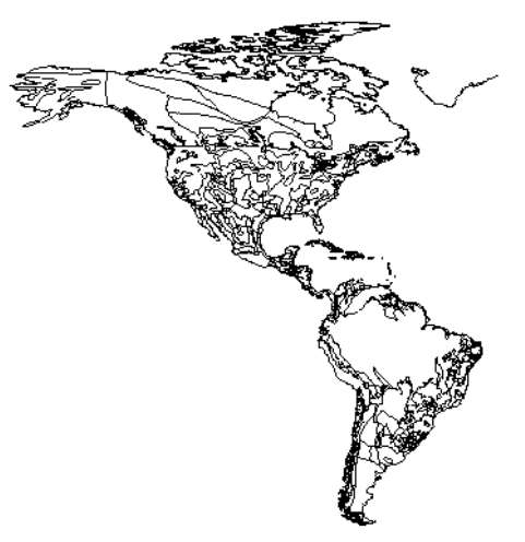
While conductivity data bases in a variety of forms can be used, in this case study a computer file of conductivity data was used. The FCC M3 Map Data File supplied by the FCC through NTIS contains two different sets of data files describing ground conductivity boundaries. The FCC M3 files, covering Canada, the United States, and Mexico are topologically organized, with conductivities defined for the west and east sides of the line segments.
The WHEM files, used in this case study, cover the entire Western Hemisphere. This data set is not organized topologically. A MapBasic program was used to convert the data into a sequence of line segments, each described by two sets of longitude and latitude coordinates and the two conductivity values on either side of the line segment. Conductivity values in mhos per meter were aggregated into eight discrete levels. This data base is stored in the WHEMSEGS table. Figure 1 shows the extent of this Western Hemisphere conductivity data base.
Noise and Interference
Acquisition and tracking are primarily functions of received signal strength with respect to atmospheric noise and man-made interfering signals. SNR is a function of transmitter power, the range and effective impedance of the propagation path, and the combination of noise and interference at the receiver location.
Read also: Loran-C Charts and Related Information
For this case study noise values were computed from CCIR noise values and stored as regions with noise value attributes in rms noise levels in decibels above one microvolt per meter in the NOISE table. No modeling of individual man-made interferers was included.
Receiver Model
The user can specify a number of receiver modes. With the ease of programming the MapBasic script language, almost any conceivable receiver model can be accommodated. The maximum number of tracked signals and chains, minimum SNRs for acquisition and tracking, and different positioning algorithms can be easily selected or reprogrammed.
The basic model is an n-chain, n-station model with user selectable minimum SNR. The user defines the position accuracy requirement for the coverage chart.
Coverage Grid
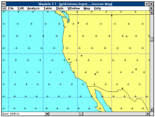
After initialization the user is presented with a world map showing the currently defined Loran-C transmitters. Using zoom tools the user selects an area for coverage prediction. When DoMap is activated a grid of points is produced by the MAKEGRID module. Grid points are produced at equal distances over the selected area. By using equal distance for grid points, rather than equal increments of degrees, the grid remains representative at higher latitudes (Figure 2).
A new impedance table, SEGMENTS, is produced containing the line segments within a defined range limit of the grid. This is done using buffering commands and SQL selections.
Ray Path Modeling
At each grid position used in the model, a ray path is computed from transmitter to receiver. This path is modeled as a polyline following the geodetic groundwave path over the earth and is stored in the table RAYPATH.
Simplified paths following a great circle route can be computed, or more complex models, describing the path over an ellipsoidal earth can be used.
Transmitter Site Conductivity Level
The WHEM conductivity data base is not topologically organized. The two conductivity values in the data base are those on either side of the boundary line, but there is no east-west (as there is in the FCC M3 files), left-right, or other fixed order to the two values. Because MapInfo has limited capabilities for building topological relationships (as do other GIS products such as ARC/INFO), the conductivity level at each transmitter site is computed whenever the transmitter data base is changed.
This is accomplished by the use of a table of known positions outside of the land conductivity boundaries. These known points at sea, stored in the SEAPOINTS table, are assumed to have a conductivity of 5,0 mhos per meter. A line from each transmitter to the nearest of these points is computed. An SQL query determines the list of line segments intersected by this line. The same SQL statement orders the intersections by range from the known sea point.
Starting from the known conductivity level of the sea point, each intersection is examined and the level on each side of the intersection determined, until the conductivity level at the transmitter site is resolved. This transmitter site conductivity level is stored in the XMITRS table.
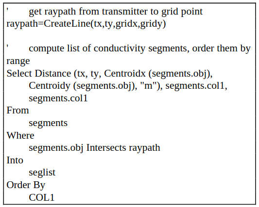
Path Impedance
The ray path polyline and the conductivity SEGMENTS table are used in an SQL query to select the conductivity boundary segments and their associated conductivity level numbers. The SQL query (Figure 3) orders the segments by distance from the transmitter.
Using the computed conductivity level at the transmitter the program computes the topological relationships for each intersecting line segment, resolving the conductivity of each path segment. Given the list of ranges and conductivities stored in the SEGLIST table, any method, from full integral solutions to Exploring Loran-C Millington’s MethodMillington’s method, can be employed for ray path field strength attenuation.
This case study uses an average impedance method that has been used for prediction of both field strength and phase delay computations.
Conductivity levels are converted to impedance values:
where:
- ∇2 – real impedance;
- n – index of refraction of air = 1,000338;
- ε0 – permittivity of free space = 8,85e-12;
- ε2 – permittivity of path (80 sea, 15 land);
- σ – conductivity in mhos/meter;
- ω = 2πf.
For each SEGLIST table, the effective path impedance is computed:
Field Strength
Field strength is a function of range, path impedance, and transmitter power. At each grid point field strength is computed for each transmitter.
A field strength value is interpolated from a table of field strength attenuation at selected ranges and impedances. That value is adjusted for transmitter power and converted to dB above one microvolt per meter.
Noise and SNR. The noise level is computed from the NOISE table as the nearest modeled noise value. SNR in decibels is computed for each transmitter by subtracting the noise level region from the field strength.
Bias Errors. Estimates for the magnitude of chain and transmitter timing bias were used in position error estimates. Values of 25 ns for chain, and 20 ns for transmitter errors were used in the case study. For this study of repeatable accuracies, no propagation model error bias was included.
ECD and Skywave. Pulse shape distortions may affect the probability of acquisition and the correct cycle identification required by Loran-C receivers to resolve ten microsecond arrival-time ambiguities. Variations in the impedance and terrain of the ground-wave path result in envelope to cycle distortion (ECD), and interference from sky-wave signals can further distort the ground-wave pulse shape. In the case study no ECD or skywave modeling was implemented, but for users requiring coverage at high geomagnetic latitudes or at long ranges, such modeling would be useful.
TOA Variance
If the SNR for a transmitter is above the minimum required for acquisition and tracking by the receiver model, a time of arrival variance is computed. The TOA variance is based on SNR, the GRI, and values for chain and transmitter timing and receiver servo bandwidth (ten second averages in the nominal model).
where:
- C – 299,69 m/μs;
- – noise to signal ratio;
- Bs – servo bandwidth in radians per second;
- Fs – samples per second;
- t1 – chain timing error = 25 ns;
- t2 – transmitter timing = 20 ns.
The resulting TOA variance is used as a weight in the position error computation:
Directional Derivatives
At each grid location the geodetic azimuth from the receiver position to each tracked transmitter is used to form the directional derivatives of range errors with respect to easting, northing, and clock errors.
The resulting matrix for n-stations is:
Position Error
Position error at a given location is computed using the following operations where the weight matrix is formed from a column of TOA variances.
GDOP
For GDOP coverage charts, the weights containing TOA variances are not used and the directional derivatives compute GDOP from:
Coverage Contours
To compute error contours a new grid is produced with four times the number of points as in the original grid. Grid points between original points are interpolated from neighboring points. Coverage contours are computed by selecting those grid points from the new grid with error estimates below the required user position accuracy.
Using an SQL statement (Figure 4) a buffer is created around the ensemble of selected grid points.
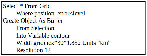
The resulting polygon is used as a contour line representing the limits of coverage for the specified position error.
Coverage Map Creation. The coverage contour is added as a layer on the user defined coverage map. The user can then select any projection and datum and prepare the map for output using the MapInfo Layout commands. Maps can be colored and annotated in a variety of ways. The resulting map can be printed, plotted, transferred to a word processor or other Windows program, or stored for later use.
Problems
MapInfo is not a highly sophisticated GIS package. The design of the LCModel program was hampered by the limited ability of MapInfo to build topological relationships from boundary lines and attributes.
Currently no capability exists in MapInfo for the conversion of connected polylines into regions. While distances are computed over great circle paths, lines created between two geodetic positions are modeled as lines in an orthogonal system of latitude and longitude coordinates, rather than as great circle or ellipsoidal paths. The lack of built-in contouring functions hampered the creation of smoothed coverage limit lines in the LCModel program.
Sample Coverage Chart
To demonstrate the capabilities of the GIS approach to modeling Loran-C coverage, the US West Coast Chain, GRI 9940, was modeled. The receiver model used is a single chain, four station receiver capable of tracking at -9 dB SNR.
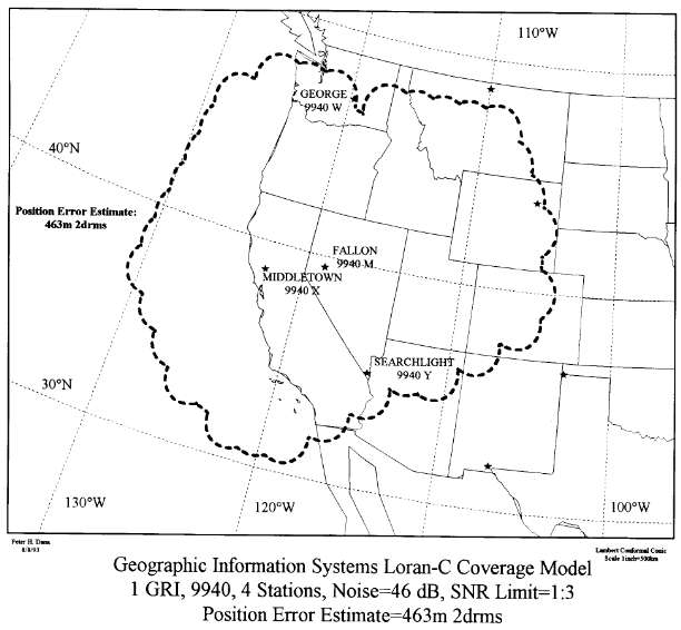
The differences between this and published coverage maps using the same coverage criteria are minimal.
GIS Spatial Analysis
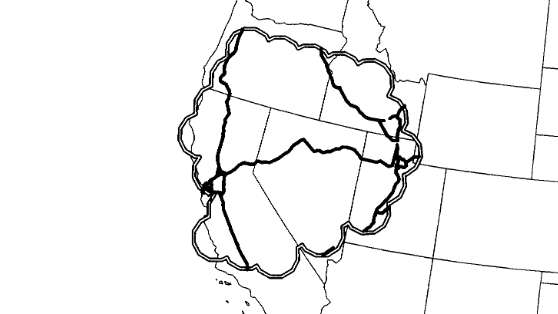
The primary advantage of GIS modeling is the ability to combine layers of data and investigate interrelationships between them. To provide a simple example, a table containing US Interstate Highways was imported into MapInfo. A SQL statement using the Sum and ObjectLen functions, computed the length of the highway system (Figure 6).
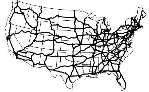
A 100 meter coverage contour was produced for a single chain receiver operating on the 9940 chain. An SQL selection was performed on the contour table and the highway table, resulting in a new table containing the highways within the contour region. Another query computed the total length of the highways within the 100 meter, 2 drms, coverage region (Figure 7).
Conclusion
Geographic information systems can provide a flexible, interactive, and adaptable means of providing Loran-C coverage estimates based on the specific requirements of independent users around the world. Providing a means of acquisition, management, analysis, and display of Loran-C system data, modern GIS packages are available for a variety of hardware platforms.
Drivers are available for hundreds of input and output devices. GIS can produce high quality output of coverage charts in map projections and geodetic datums required by a variety of users.
Of particular significance is capability of GIS to model interoperable navigation systems. GIS techniques offers the potential for modeling differential GPS (DGPS) coverage and Loran-C concurrently, enabling independent users to experiment with DGPS beacon placement within existing and proposed Loran-C transmitter coverage.
A fundamental advantage of GIS methods is the ability to use Loran-C coverage predictions in conjunction with other layers of spatial information. Rapid advances in GIS technologies will provide additional Loran-C coverage modeling capabilities in the future.

- Jansky & Bailey. The Loran-C System of Navigation. Alexandria, VA: Jansky and Bailey, Atlantic Research Corporation. 1962.
- US Coast Guard. Loran-C User Handbook CG-462. Washington, DC: U.S. Department of Transportation. 1974.
- US Coast Guard. Loran-C User Handbook COMDTINST MI6562.3. Washington, DC: U.S. Department of Transportation. 1980.
- US Coast Guard. Specification of the Transmitted Loran-C Signal MI6562.4. Washington, DC: U.S. Department of Transportation. 1981.
- El-Arini, M. B. Airport Screening Model for Nonprecision Approaches Using Loran-C Navigation. McLean, VA: The Mitre Corporation. 1984.
- Bleau, Charles A. and Franklin MacKenzie. Model for Forecasting Loran-C Coverage. Proceedings of the Thirteenth Annual Technical Symposium. Bedford, MA: The Wild Goose Association. 1984.
- Last, David, Richard Farnsworth, and Mark Searle. A European Loran-C Coverage Prediction Model. Proceedings of the Nineteenth Annual Technical Symposium. Bedford, MA: The Wild Goose Association. 1990.
- Catlin, Jeff, Dean Foulis, Gary Noseworthy, and Gene Allard. The Automated Loran-C Coverage Diagram Generator. Proceedings of the Eighteenth Annual Technical Symposium. Bedford, MA: The Wild Goose Association. 1989.
- US Coast Guard. Loran-C User Handbook COMDTPUB P16562.6. Washington, DC: U.S. Department of Transportation. 1992.
- Federal Aviation Administration. Advisory Circular 90-92. Washington, DC: U.S. Department of Transportation, General Services Section. 1993.
- Last, David, Mark Searle, and Richard Farnsworth. Coverage and Performance Predictions for the North-West European Loran-C System. Proceedings of the Twenty-First Annual Technical Symposium. Bedford, MA: The Wild Goose Association. 1992.
- FCC. FCC M3 Map Data File PB81-211567. Springfield, VA: National Technical Information Service. 1981.
- CCIR. World Distribution and Characteristics of Atmospheric Radio Noise, CCIR 322. Geneva: International Telecommunications Union, International Radio Consultative Committee. 1963.
- Penrod, Bruce, Richard Funderburk, and Peter Dana. Arrival of Loran-C Transmissions via GPS Common Mode/Common View Satellite Observations. Proceedings of the National Technical Meeting. Washington, DC: The Institute of Navigation. 1991.
- Kayton, Myron and Walter R. Fried, eds. Avionics Navigation Systems. New York: John Wiley & Sons. 1969.