Mathematical Model used for the Vessel Simulator Tool

To be able to validate a simulation model, the mathematical model used for describing the forces and motion of the vessel have to be properly documented. An introduction to the elementary ship motions, the reference frame used for ship manoeuvring and a description of the basic 3-DOF model will be addressed. This will be followed by a descriptive overview of the mathematical model used for the simulation tool Vessel Simulator (VeSim).

СодержаниеСвернуть

Motions and axis system
Linear 3-DOF model
Dynamically stable vessel
Structure of VeSim
HullVisc
Vessel Model (VeSim)
Non-dimensional coefficients
Nomenclature
Greek symbols

Motions and axis system

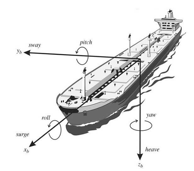
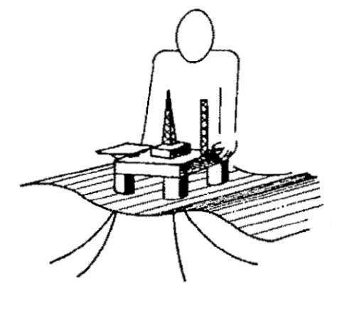
A ship experiences motion in 6 degrees of freedom (DOF). The DOF describe the independent displacements and rotations of the ship. The motions in the horizontal plane are referred to as surge (longitudinal motion), sway (sideways motion) and yaw (rotation about the vertical axis) and describes the heading of the ship. The last three DOF are roll (rotation about the longitudinal axis), pitch (rotation about the transverse axis) and heave (vertical motion). See Picture 1.

For development of mathematical models for ships there exist various approach methods. Manoeuvring theory states that a ship moving in restricted, sheltered water can be described with a linear 3-DOF (surge, sway and yaw) equation based on Newton’s second law. Newton’s second law is given as

\vec{F} = m \vec{a}

, and states that the alteration of motion is proportional to the motive force impressed; and is made in the direction of the right line in which that the force is impressed. The manoeuvring model is derived for a ship moving with the velocity U in a positive direction, with a zero-frequency wave excitation. This enables the added mass and damping to be represented by the use of hydrodynamic derivatives (constant parameters). The motions are given relative to a body fixed reference frame, see Picture 1 for visualization.

Note! The zero-frequency assumption is only valid for surge, sway and yaw.

This linear approximation is the simplest representation of a manoeuvring model. A non-linear approximation can be derived using an Euler-Lagrangian approach, cross-flow drag, quadratic damping or a Taylor-series expansion. The non-linear approximation uses a 6 DOF model (surge, sway, heave, roll, pitch and yaw) which is a fully coupled equation of motion.

Nomenclature for all the formulas you can see here: Nomenclature and Greek Symbols

It is desirable to derive the equations of motion for a ship from an arbitrary point, CO. This is to take advantage of the vessel’s geometric properties. The hydrodynamic forces and moments are often computed in CO. The point CO is specified by the control engineer and is commonly located on the centreline midships as seen in Picture 1.

The forces and moments are listed in Table 1 and the nomenclature follows the SNAME and ITTC standard used for manoeuvring problems.

Table 1. Forces and motion parameters in manoeuvring
DOF	Motion type		Forces and moments	Linear and angular velocities
1	Linear x-axis	Surge	X	u
2	Linear y-axis	Sway	Y	v
3	Linear z-axis	Heave	Z	w
4	Rotation about x-axis	Roll	K	p
5	Rotation about y-axis	Pitch	M	q
6	Rotation about z-axis	Yaw	N	r

Linear 3-DOF model

When using the linear 3-DOF model, only the motions in the horizontal plane (surge, sway and yaw) are evaluated in the mathematical equation. The relationship between the forces from the fluid and the motion of the vessel can be derived from Newton’s second law and given as:

\frac{d}{d t} (M {\vec{U}}_{A}) = {\vec{F}}_{1} E q . 1

where:

The hydrodynamic forces and control forces from rudders are included in the force ${\vec{F}}_{1}$ ;
The absolute velocity in the centre of gravity is given as ${\vec{U}}_{A}$ and M is the mass of the body.

The rotational equation of motion can be expressed as:

\frac{d}{d t} {(I \vec{ω})}_{G} = {\vec{F}}_{2} E q . 2

where:

The hydrodynamic moments and control moments from rudders are included in the moment ${\vec{F}}_{2}$ ;
The moment of inertia-matrix is given as I and $\vec{ω}$ is the rotation;
The equation applies to an axis system with origin in the hull’s centre of gravity, indicated by the index G.

This gives rise to equations of motions expressed as:

\begin{matrix} X = M \dot{u} \\ Y = M (\dot{v} + x_{G} \dot{r} + u r) \\ N = I_{z z} \dot{r} + M x_{G} (\dot{v} + u r) \end{matrix} E q . 3

where:

x_G – is the distance between the vessel’s centre of gravity and the origin in the axis system;
I_zz – is the moment of inertia about the vertical axis, through the midship point (CO).

When the Introduction to the Standard Simulation Tests and Requirements for Naval Hydrodynamicshydrodynamic hull forces and control forces from the rudder are included, the following linear equations of motions are given:

\begin{matrix} (X_{\dot{u}} - M) \dot{u} = 0 \\ (Y_{\dot{v}} - M) \dot{v} + (Y_{\dot{r}} - M x_{G}) \dot{r} + Y_{v} v + (Y_{r} - M u) r + Y_{δ} δ = 0 \\ (N_{\dot{v}} - M x_{G}) \dot{v} + (N_{\dot{r}} - I_{z z}) \dot{r} + N_{v} v + (N_{r} - M x_{G} u) r + N_{δ} δ = 0 \end{matrix} E q . 4

With this linear equation, no speed loss is predicted. For this reason, the linear equation can only be valid when:

The vessel has straight line stability;
There is straight line motion at constant speed.

The sway and yaw equations (4), can be made dimensionless by dividing the expressions by

\frac{1}{2} ρ L_{p p}^{2} U^{2}

and

\frac{1}{2} ρ L_{p p}^{3} U^{2}

, respectively.

The non-dimensional sway and yaw equations are then expressed as:

\begin{matrix} (Y_{\dot{v}}^{'} - M^{'}) {\dot{v}}^{'} + (Y_{\dot{r}}^{'} - M^{'} x_{G}^{'}) {\dot{r}}^{'} + Y_{v}^{'} v^{'} + (Y_{r}^{'} - M^{'}) r^{'} + Y_{δ}^{'} δ = 0 \\ (N_{\dot{v}}^{'} - M^{'} x_{G}^{'}) {\dot{v}}^{'} + (N_{\dot{r}}^{'} - I_{z z}^{'}) {\dot{r}}^{'} + N_{v}^{'} v^{'} + (N_{r}^{'} - M^{'} x_{G}^{'}) r^{'} + N_{δ}^{'} δ = 0 \end{matrix} E q . 5

where:

′ – denotes that the parameter is dimensionless.

Dynamically stable vessel

By introducing a differential operator

D = \frac{d}{d t}

, the straight line stability of a vessel can be investigated. The accelerations are written as:

\begin{matrix} {\dot{v}}^{'} = D v^{'} \\ {\dot{r}}^{'} = D r^{'} \end{matrix} E q . 6

Equation (5) can thereby be re-written as:

\begin{matrix} ((Y_{\dot{v}}^{'} - M^{'}) D + Y_{v}^{'}) v^{'} + ((Y_{\dot{r}}^{'} - M^{'} x_{G}^{'}) D + (Y_{r}^{'} - M^{'})) r^{'} + Y_{δ}^{'} δ = 0 \\ ((N_{\dot{v}}^{'} - M^{'} x_{G}^{'}) D + N_{v}^{'}) v^{'} + ((N_{\dot{r}}^{'} - I_{z z}^{'}) D + (N_{r}^{'} - M^{'} x_{G}^{'})) r^{'} + N_{δ}^{'} δ = 0 \end{matrix} E q . 7

The sway velocity term may be eliminated by:

Multiplying the sway equation with
$((N_{\dot{v}}^{'} - M^{'} x_{G}) D + N_{v}^{'});$
Multiplying the yaw equation with
$((Y_{\dot{v}}^{p} - M^{p}) D + Y_{v}^{p});$
Subtracting the resulting sway equation from the yaw equation.

The result is given by:

(A D^{2} + B D + C) r^{'} = (E D + F) δ E q . 8

where (this is Equation 9):

$A = (N_{\dot{r}}^{p} - I_{z z}^{p}) (Y_{\dot{v}}^{p} - M^{p}) - (Y_{\dot{r}}^{p} - M^{p} x_{G}^{p}) (N_{\dot{v}}^{p} - M^{p} x_{G}^{p});$
$B = (N_{\dot{r}}^{'} - I_{z z}^{'}) Y_{\dot{v}}^{'} + (N_{r}^{'} - M^{'} x_{G}^{'}) (Y_{\dot{v}}^{'} - M^{'}) - (Y_{\dot{r}}^{'} - M^{'} x_{G}^{'}) N_{v}^{'} - (Y_{r}^{'} - M^{'}) (N_{\dot{v}}^{'} - M^{'} x_{G}^{'});$
$C = (N_{r}^{'} - M^{'} x_{G}^{'}) Y_{v}^{'} - (Y_{r}^{'} - M^{'}) N_{v}^{'};$
$E = Y_{δ}^{'} (N_{\dot{v}}^{'} - M^{'} x_{G}^{'}) - N_{δ}^{'} (Y_{\dot{v}}^{'} - M^{'});$
$F = Y_{δ}^{'} N_{\dot{v}}^{'} - Y_{δ}^{'} Y_{\dot{v}}^{'} .$

Equation (8) is a first order differential equation, where the yaw speed can be written as:

r^{'} (t^{'}) = r_{H}^{'} + r_{P}^{'} = C_{1} e x p (D_{1} t^{'}) + C_{2} e x p (D_{2} t^{'}) + r_{P}^{'}, E q . 10

where:

$r_{H}^{'}$ – is the homogeneous solution and;
$r_{P}^{'}$ – is the particular solution.

Setting the rudder angle to zero, the homogeneous solution

r_{H}^{'}

, can be calculated using:

\begin{matrix} A D^{2} + B D + C = 0 \\ D_{1, 2} = \frac{- B \pm \sqrt{B - 4 A C}}{2 A} \end{matrix} E q . 11

For a ship with straight line stability the homogeneous solution goes to zero as the time goes to infinity, which is obtained when the exponential coefficients D1,2 have real parts. This implies that in order to have straight line stability:

C > 0. Eq. 12

This is satisfied if:

\frac{N_{r}^{'} - M^{'} x_{G}^{'}}{Y_{r}^{'} - M^{'}} > \frac{N_{v}^{'}}{Y_{v}^{'}} E q . 13

Structure of VeSim

The Vessel Simulator (VeSim) model developed by MARINTEK is a time domain simulation tool. The model combines manoeuvring and seakeeping into one common simulation model.

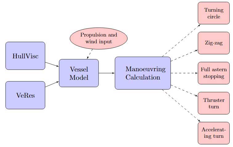
The VeSim simulation model consists of several pre-processors and input variables. HullVisc and VeRes computes the hydrodynamic properties, and the wave loads and motions in the frequency domain, respectively. These are then input to the Vessel Model along with propulsion and wind input. The Vessel Model computes the vessel motions and retardation functions in the time domain along with the Information about Vessel Manoeuvring based on IMO Standardsmanoeuvring forces. The user can then calculate the different calm water manoeuvres. The flow of the total model is graphically presented in the flowchart in Picture 2 below.

Definition of coordinate systems in VeSim

The simulation model (VeSim) applies in total, three different reference frames. The NED-frame and the body-frame, which are applied when calculating the ship motions. And the naval-frame, which is used for describing the positions on the vessel.

The north-east-down (NED) reference frame is defined relative to the Earth’s ellipsoid, see Picture 3.

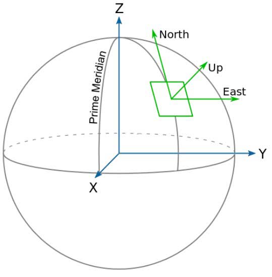
North-east-down frame — Pic. 3 NED-frame

The x_n-axis is positioned along the northern axis, the y_n-axis is directed towards the east and to uphold the right-hand rule, the z_n-axis is directed downwards, towards the center of the Earth. The NED-frame is used when the computations of the motions are performed.

The body-frame is fixed to the vessel. The origin of this frame is fixed in the center of gravity of the vessel. The x_b-axis is directed towards the bow, the y_b-axis is directed towards starboard and to uphold the right-hand rule, the z_b-axis is directed downwards. This is the same reference frame which is depicted in Picture 1. The body-frame is used when describing the cross-sectional geometry of the vessel and when calculating the external forces on the vessel.

The naval-frame is used to describe positions on the vessel and is commonly used in design and naval architecture, hence the term naval-frame. Unlike the previous reference frames, this frame is a left-handed system. The origin of the frame is located at the intersection between the aft perpendicular (AP), the centreline (CL) and the base line (BL) of the vessel. The x-axis is directed forwards, towards the bow. The y-axis is directed towards starboard and the z-axis is then directed upwards. The naval-frame is used for the graphical interface in ShipX.

HullVisc

The hydrodynamic coefficients have been calculated using ShipX. ShipX is an inter- face program that allows the user to analyse the ship at an early design stage. ShipX uses amongst others, an additional plug-in for manoeuvring prediction called SIMAN. SIMAN uses a pre-processor called HullVisc to calculate the hydrodynamic coefficients. HullVisc allows the user to predict the hydrodynamic coefficients on the basis of the ship’s geometry, which is accessible in the early stages of design.

Strip theory

A combination of slender body and strip theory is used to describe the acceleration dependent forces and moments excited during the calm water manoeuvre. Lighthill’s theorem is used to calculate the linear velocity dependent forces and moments with a sectional distribution of the added mass. HullVisc compare results from model tests of approximately 25 different ships, the calculations are modified using expressions based on regression analysis of these models.

HullVisc uses an uneven distribution of the hull sections, concentrating the number of sections at the fore part of the ship and in the aft. This is to get a more correct measurement in these parts of the ship, as they include more complicated lines than the mid-section. The hull’s cross sections are increased along the ship’s length, from bow to the stern. This is to give the hull a more realistic boundary layer. It will also give a correction at the stern for the full body forms when using slender body theory.

The forces derived from Lighthill’s theorem are adopted by John Nicholas Newman in “Marine Hydrodynamics” and Odd Magnus Faltinsen in “Hydrodynamics for high speed marine vehicles”. It should be mentioned that Lighthill uses a different notation from what is used in the ITTC/SNAME standard.

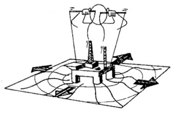
By evaluating a slender fish moving in the water, Lighthill stated that the force in heave (equivalent to sway, see Picture 4) can be described as:

f_{3}^{H D} = - (\frac{\partial}{\partial t} + U \frac{\partial}{\partial x}) [a_{33} (\frac{\partial w}{\partial t} + U \frac{\partial w}{\partial x})] E q . 14

Where a₃₃ is the two-dimensional infinite-frequency added mass in heave. But because a ship-fixed coordinate system is used, the term

U \frac{\partial w}{\partial x}

does not appear. By evaluating equation (14) in a manoeuvring aspect, the equation can be expressed as:

f_{2}^{H D} = - (\frac{\partial}{\partial t} + U \frac{\partial}{\partial x}) [a_{22} ({\dot{n}}_{2} + x {\dot{η}}_{6})] E q . 15

where:

$f_{2}^{H D}$ – is the two-dimensional horizontal force on the hull;
η – is the vessel motion in the direction of the subscripts 2 and 6, given as sway and yay, respectively;
$\dot{η}$ and $\ddot{η}$ represents the velocity and acceleration for the respective motions;
a₂₂ – is the low-frequency two dimensional added mass in sway.

The total force acting on the body can be obtained by strip-theory and integration over the length of the ship.

The following hydrodynamic sway force is obtained:

F_{2}^{H D} = [\int_{L} a_{22} d x {\ddot{η}}_{2} + \int_{L} a_{22} x d x {\ddot{η}}_{6} + U a_{22} (x_{T}) {\dot{η}}_{2} + U x_{T} a_{22} (x_{T}) {\dot{η}}_{6}] E q . 16

Where x_T is the x-coordinate of the transom stern. Similarly, by multiplying equation (16) by the moment arm x, and integrating over the length of the ship, the yaw moment is found.

F_{6}^{H D} = - \{\int_{L} x a_{22} d x {\ddot{η}}_{2} + \int_{L} a_{22} x^{2} d x {\ddot{η}}_{6} + U \{[x_{T} a_{22} (x_{T}) - \int_{L} a_{22} d x] {\dot{η}}_{2} + [x_{T}^{2} a_{22} (x_{T}) - \int_{L} x a_{22} d x] {\dot{η}}_{6}\}\} E q . 17

Equation (16) and (17) give the sway force and yaw moment acting on the hull according to the slender body theory. Table 2 shows the Hydrodynamic coefficients derived from Lighthill’s theorem of a swimming slender fish compared with the standard notation of the manoeuvring forces and the slender-body theory.

Table 2. Hydrodynamic forces based on slender body theory
Notation from Newman	Standard Notation	Slender body theory
∂F₃/∂U₃	Y_v	-Ua₂₂(x_T)
∂F₃/∂Ω₂	-Y_r	-Ux_ta₂₂(x_T)
$\partial F_{3} / \partial {\dot{U}}_{3}$	$Y_{\dot{v}}$	$- \int_{L} a_{22} d x$
$\partial F_{3} / \partial {\dot{Ω}}_{2}$	$- Y_{\dot{r}}$	$- \int_{L} x a_{22} d x$
∂M₂/∂U₃	-N_v	$U [\int_{L} a_{22} d x - x_{T} a_{22} (x_{T})]$
∂M₂/∂Ω₂	N_r	$U [\int_{L} x a_{22} d x - x_{T}^{2} a_{22} (x_{T})]$
$\partial M_{2} / \partial {\dot{U}}_{3}$	$- N_{\dot{v}}$	$- \int_{L} x a_{22} d x$
$\partial M_{2} / \partial {\dot{Ω}}_{2}$	$N_{\dot{r}}$	$- \int_{L} x^{2} a_{22} d x$

x_T – denotes the added-mass coefficient at the stern;
a₂₂, xa₂₂ and x²a₂₂ is the sway added-mass coefficient, the cross-coupling added-mass between sway and yaw, and the added moment of inertia for yaw acceleration, respectively;
U, U₃ and Ω₂ is the non-zero velocity components of the ship in forward, sway and yaw motion, respectively.

In Picture 4 the notation used by Newman describes x as positive forward, y upward and z to starboard.

Newman notation and standard notation — Pic. 4 The notation used by Newman, a) and standard notation, b)

The velocity components are U₁, U₃ and Ω₂ which denotes forward, sway and yaw velocity, respectively. F₃, M₂ and δ_R is defined as the sway force, yaw moment and rudder angle, respectively. As Picture 4 illustrates, this differs from the standard notation given by figure b). Here, z is positive downward, x forward and y towards starboard. X and Y is the hydrodynamic force components along the x– and y-axis, and N is the hydrodynamic yaw-moment about the z-axis. u, v, r and δ is the longitudinal, lateral, yaw angular velocity and rudder angle, respectively.

HullVisc Results

The input data specified in SIMAN are shown in Table 3.

Table 3. Input data to SIMAN
Definition	Nomenclature	Units
Draught	T = 3,6	m
Length	Lpp = 90	m
Breadth	B = 16,81	m
Displacement	∇ = 2 494,634	m³
Block coefficient	C_B = 0,396	[-]
Weight	∆ = 2 557	tons
Speed	V = 19	knots

The resulting hydrodynamic coefficients calculated by HullVisc are tabulated in Table 4.

Table 4. Hydrodynamic coefficient from HullVisc
$Y_{v}^{'}$	-0,00539 [-]	$Y_{\dot{v}}^{'}$	-0,00353 [-]
$Y_{r}^{'}$	0,00182 [-]	$Y_{\dot{r}}^{a}$	0,00018 [-]
$N_{v}^{'}$	-0,00140 [-]	$N_{\dot{v}}^{'}$	0,00018 [-]
$N_{r}^{'}$	-0,00072 [-]	$N_{\dot{r}}^{a}$	-0,0026 [-]

Validity of HullVisc

The Vessel Response (VeRes) processor can be divided into two different main processes. The first and the most important for the intended simulations, is the process which calculates the transfer functions for the vessel motions and loads, given in a frequency domain. It may also perform time simulations. The second process is a post-processor which enables the user to make reports and presentations of the data. Further calculations based on the transfer functions may also be carried out.

Some of the main VeRes calculations that the first process can carry out are listed below:

Motion transfer functions in 6-DOF;
Relative motion transfer functions;
Motion transfer functions at specified points;
Global wave induced loads given by forces and moments;
Time simulations of motions and loads including important non-linear effects.

When calculating ship motions and loads, general assumptions and simplifications are made. Computer programs used to calculate and estimate these forces and motions are configured with such simplifications. The user must be aware of the simplifications used by the program and be able to validate the results by knowing the limitations and restrictions of the computer software. The main assumptions in VeRes are the use of linear, potential and strip theory.

The main simplifications and assumptions applied in VeRes are listed below:

The ship is oscillating with the same frequency as the wave encounter frequency.
Linearity is assumed between the responses and the incident wave amplitude because of linear theory.
The loads and motions on a vessel in a sea state is derived by use of the superposition principle.
Potential theory is applied when evaluating sea loads and motions. Potential theory states that the fluid is incompressible, inviscid, homogeneous and irrotational. Empirical formulas are used when accounting for viscous roll damping.
Slender-body theory is assumed, which states that the length of the ship is much larger than the breadth and draught (L >> B, T).
Strip theory is applied in the frequency domain when evaluating hydrodynamic problems. The ship is divided into small two-dimensional cross sectional strips and integrated along the ship length to obtain three-dimensional values.
The vessel is assumed to be symmetric about its centreline.

Equation of motion

VeRes is primarily based upon linear strip theory. The main assumptions for linear theory are:

The velocity potential is proportional to the wave amplitude and is valid if the amplitude is small relative to a characteristic wavelength and body dimension.
The wave steepness is small, i. e. the waves are far from breaking.

In “Sea Loads on Ships and Offshore Structures” by O. M. Faltinsen it is stated that:

By adding together results from regular waves with different amplitudes, wave-lengths and propagation directions, it is possible to obtain results of irregular waves.

If the ship is analysed in incident regular sinusoidal waves of small wave steepness, this will be sufficient from a hydrodynamical point of view.

Further, if steady state conditions are assumed, i. e. there are no transient effects present due to initial conditions, the linear dynamic motions and loads are harmonically oscillating with the same frequency as the wave loads that excite the ship (the same frequency as the wave encounter frequency). This will allow for computations in the frequency domain.

The encounter frequency, ω, is given from the relation:

ω = ω_{0} + \frac{ω_{0}^{2} U}{g} \cos β E q . 18

where:

ω₀ – is the wave frequency;
U – is the forward velocity of the vessel;
β – is the angle between the vessel and the wave propagation direction and;
g – is the acceleration of gravity.

If the responses are assumed to be linear and harmonic, the linear coupled differential equation of motion for the six degrees of freedom can be written as:

\sum_{k = 1}^{6} [(M_{j k} + A_{j k}) {\ddot{η}}_{k} + B_{j k} {\dot{η}}_{k} + C_{j k} η_{k}] = F_{j} e^{i ω t}, j = 1, . . . . ., 6 E q . 19

where:

M_jk – represents the elements of the generalized mass matrix.
A_jk – represents the elements of the added mass matrix.
B_jk – represents the elements of the linear damping matrix.
C_jk – represents the complex of the stiffness matrix.
F_j – represents the complex amplitudes of the wave exciting forces and moments, with the physical forces and moments given by the real part of F_je^iωt. F₁, F₂, F₃, F₄, F₅ and F₆ refer to the amplitudes of the surge, sway and heave exciting forces and the amplitudes of the roll, pitch and yaw exciting moments, respectively.
ω – is the angular frequency of encounter.
η_k – represents surge, sway, heave, roll, pitch and yaw motion amplitudes, respectively. The dots and double dots denotes time derivatives, and are velocity and acceleration terms, respectively.

The different contributions to the equations of motion are the mass forces due to the mass of the vessel, and follows directly from Newton’s law. This can be expressed in terms of the motion of the ship, η_k, as:

F_{j} = - M_{j k} {\ddot{η}}_{k} E q . 20

where:

M_jk – are the components of the generalized mass matrix for the ship.

The steady-state added-mass and damping forces are due to forced harmonic rigid body motions when there are no incident waves. The forced motion of the vessel generates outgoing waves and oscillating fluid pressures on the hull surface. By integration of these fluid pressure forces over the wetted body surface of the hull, the resulting forces and moments on the body are obtained. These forces and moments are proportional to the body acceleration and velocity. The hydrodynamic added mass and damping loads due to the harmonic motion mode, η_k, can be written as:

F_{j} = A_{j k} {\ddot{η}}_{k} E q . 21

where:

A_jk and B_jk are the added mass and damping coefficients, respectively.

The restoring forces and moments, which are body geometry and mass distribution dependent, can be written as:

F_{j} = - C_{j k} η_{k} E q . 22

where:

C_jk – are the restoring coefficient.

Picture 5 depicts the concept of the added mass, damping, and restoring forces and moments.

Scheme: motion — Pic. 5 Added mass, damping and, restoring forces and moments

The linearized wave exciting forces and moments are the loads on the body when the body is restrained from oscillating and there are incident waves present. These forces are divided into Froude-Kriloff and diffraction forces. The Froude-Kriloff force is the force excited on the vessel due to the undisturbed pressure field on the body, which again is induced by the unsteady pressure of the undisturbed waves. The diffraction force is the additional force because of the fact that the body changes this pressure field.

The motion transfer functions are then given by the amplitude η_a, and phase angle θ, and defined as:

η_{k} (t) = η_{k a} \cos (ω t + θ_{k}), k = 1 . . . . . 6 E q . 23

Picture 6 depicts the concept of the linearized wave excitation forces and moments.

Viscous roll damping

When predicting the roll motions, viscous roll damping from the hull and bilge keels are included. The roll equation of motion is written as:

(M_{42} + A_{42}) {\ddot{η}}_{2} + B_{42} {\dot{η}}_{2} + (M_{44} + A_{44}) {\ddot{η}}_{4} + (B_{44}^{P} + B_{44}^{V_{1}}) {\dot{η}}_{4} + B_{44}^{V_{2}} | {\dot{η}}_{4} | {\dot{η}}_{4} + C_{44} {\dot{η}}_{4} + (M_{46} + A_{46}) {\ddot{η}}_{6} + B_{46} {\dot{η}}_{6} = F_{4}, E q . 24

where:

The the potential, linear and quadratic viscous damping terms are denoted by the superscripts P, V₁ and V₂, respectively.

The quadratic viscous damping term makes the equation non-linear and is solved by iteration. The viscous roll damping components taken into consideration by VeRes, are as follows:

Frictional damping caused by skin friction stresses on the hull;
Eddy damping caused by pressure variation on the naked hull;
Bilge keel damping.

Vessel Model (VeSim)

Hydrodynamic properties of the vessel and the wave induced vessel responses, calculated by respectively HullVisc and VeRes, are pre-processors used to calculate the retardation functions. The retardation functions are calculated in the Vessel Model plug-in for VeSim and are used to solve the vessel’s motions in 6 degrees of freedom. The Vessel Model plug-in consists of ship resistance, manoeuvring forces, added mass, damping and restoring forces, and viscous roll damping.

In addition to these pre-processors, input data is given to propulsive units and wind force. The following procedure of calculating the accelerations, velocities, motions, radiation forces and manoeuvring forces as part of the generation of the retardation functions, is a shortened and rendered edition of what presented in the VeSim documentation library.

Calculation of accelerations, velocities and motions

The 6 degrees of freedom motion responses can be obtained by assuming that the vessel is moving as a rigid body and neglecting hydroelastic effects. Given a body-fixed reference frame, the equations of motion in the time domain can be given as:

(m + A_{\infty}) \ddot{η} + C (\dot{η}) \dot{η} + D_{1} \dot{η} + D_{2} f (\dot{η}) + K η + \int_{0}^{t} h ((t - τ) \dot{η} (τ) d τ) = q (t, η, \dot{η}) E q . 25

where:

η – is the 6 degree of freedom motion vector (surge, sway, heave, roll, pitch and yaw);
m – is the body mass matrix;
A_∞ – is the added mass at infinite frequency;
C – is the coriolis;
D₁ – is the linear damping matrix;
D₂ – is the quadratic damping matrix;
f – is the vector function;
K – is the restoring matrix;
h(τ) – is the retardation function, and;
q – is the excitation forces.

The excitation forces on the right hand side of equation (25) are be given by:

q (t, η, \dot{η}) = q_{w i n d} + q_{w a v e}^{(1)} + q_{w a v e}^{(2)} + q_{p r o p} + q_{m a n} + q_{e x t} E q . 26

where:

q_wind(1) – is the wind drag force;
q_wave(2) – is the first order wave excitation force;
q_wave – is the second order wave drift force;
q_prop – is the propulsion force;
q_man – is the manoeuvring forces, and;
q_ext – is the remaining forces.

To solve for the accelerations, velocities and motions in the time domain, Newton’s second law has been applied:

M \ddot{η} = \sum_{} F_{i}

where:

M – is the 6×6 inertia matrix;
$\ddot{η}$ – is the generalized acceleration vector and;
F_i – is the lineary superimposed forces and moments vector.

By changing the nonation, Newton’s second law can be written as:

M \dot{v} = \sum_{} F_{i}

where:

v – is the generalized velocity vector and the dot symbolizes the acceleration derivative.

v = {[u, v, w, p, q, r]}^{T}

where:

The linear velocities in surge, sway and heave are given by
$(u, v, w) = ({\dot{η}}_{1}, {\dot{η}}_{2}, {\dot{η}}_{3})$
and;
The corresponding angular velocities in roll, pitch and yaw are given by
$(p, q, r) = ({\dot{η}}_{4}, {\dot{η}}_{5}, {\dot{η}}_{6}) .$

By introducing the same notation for equation (25), it can be re-written as:

(m + A_{\infty}) \dot{v} = q (t, η, v) - \int_{0}^{t} h (t - τ) v (τ) d τ - K η - D_{1} v + D_{2} f (v) + K η - C (v) v, E q . 27

with the sum of all the forces and moments being equal to:

\sum_{} F_{i} = q (t, η, v) - \int_{0}^{t} h (t - τ) v (τ) d τ - K η - D_{1} v + D_{2} f (v) + K η - C (v) v E q . 28

The accelerations can then be solved by the sum of mass and added mass divided by the sum of forces:

\dot{v} = {(m + A_{\infty})}^{- 1} \sum_{} F_{i} E q . 29

To obtain the velocities, the accelerations are integrated using an ODE1 Euler method.

Radiation forces

Radiation forces are computed by applying a convolution integral technique on the retardation functions. A convolution integral is a mathematical operation applied on two functions and producing a third function. This third function is a modified version of the original functions, giving the area overlap between the two functions. Convolution has the similar principal as that of cross-correlation.

F = \int_{0}^{t} h (t - τ) \dot{η} (τ) d τ E q . 30

By transforming the frequency-dependent added mass and damping, the retardation function can be computed:

h (τ) = \frac{1}{2 π} \int_{- \infty}^{+ \infty} [c (ω) + i ω a (ω)] e^{i ω t} d ω E q . 31

where:

$a (ω) = A (ω) - A_{\infty};$
$c (ω) = C (ω) - C_{\infty} .$

and:

A(ω) – is the frequency dependent added mass matrix;
C(ω) – is the frequency dependent potential damping matrix;
C_∞ – is the damping matrix at infinite frequency, and;
C_∞ = 0.

If the assumption of c(ω) = c(-ω), a(ω) = a(-ω), and h(τ) = 0 for τ > 0 is used, the retardation function can be rewritten as:

h (τ) = \frac{2}{π} \int_{0}^{+ \infty} c (ω) \cos ω τ d ω = - \frac{2}{π} \int_{0}^{+ \infty} ω a (ω) \sin ω τ d ω, f o r τ > 0 E q . 32

Manoeuvring forces

When addressing manoeuvring problems, the damping terms in the horizontal motions (surge, sway, yaw) and how they are determined is very important. Friction and fluid viscosity are the main sources of damping. Friction and wave resistance are the main force contributors in the longitudinal (surge) direction. While cross flow separation will be the main force acting in the transverse (sway) direction.

When addressing the vessel in its surrounding fluid, the relative velocity between the two can be expressed in terms of:

u_{D}^{(i)} = u_{w}^{(i)} (θ, x) + u_{c}^{(i)} (x) - u_{v}^{(i)} (x), i = 1, 2 E q . 33

where:

i – i = 1 for surge motion and i = 2 for sway motion;
x – is the longitudinal point of the vessel;
$u_{w}^{(i)}$ – is the wave particle velocity at the centre of buoyancy (COB) and is assumed constant along the vessel;
$u_{c}^{(i)}$ – is the current velocity;
$u_{v}^{(i)}$ – is the vessel velocity.

Longitudinal resistance in surge

The longitudinal polynomial resistance

F_{D}^{(1)}

is generated from the resistance curve, which is provided from empirical methods of vessels in calm water.

F_{D}^{(1)} = R_{0} + R_{1} u_{D}^{(1)} + R_{2} {(u_{D}^{(1)})}^{2} + R_{3} {(u_{D}^{(1)})}^{3} + . . . E q . 34

Cross flow drag forces in sway and yaw

Cross flow drag is a non-linear force, which is described as the drag force that occurs when a flow separates at the opposite side of a structure exposed to an inflowing fluid. The cross flow will generate drag forces in the opposite direction of the inflow direction and a lift force in the perpendicular direction.

The cross flow drag force on a strip can be expressed as:

f_{D}^{(2)} (θ, x) = C_{D} (θ, x) u_{D}^{(2)} (θ, x) | u_{D}^{(2)} (θ, x) | E q . 35

where:

C_D – is the cross flow drag coefficient past an infinitely long cylinder. It is computed in terms of empirical formulas.

When considering cross flow drag in sway and yaw motions, the longitudinal relative velocity components are assumed to have no effect on the transverse force.

The total cross flow drag in sway and yaw are obtained by integrating the cross flow drag force over the length of the vessel:

F_{D}^{(2)} (θ) = \frac{1}{2} ρ \int_{L} c_{D} (θ, x) D (x) u_{D}^{(2)} (θ, x) | u_{D}^{(2)} (θ, x) | d x E q . 36

F_{D}^{(6)} (θ) = \frac{1}{2} ρ \int_{L} c_{D} (θ, x) D (x) u_{D}^{(2)} (θ, x) | u_{D}^{(2)} (θ, x) | d x E q . 37

where:

C_{D} (θ, x) = \frac{1}{2} ρ c_{D} (θ, x) D (x) E q . 38

and:

i = 6 – is the superscript for yaw motion;
ρ – is the density of water;
L – is the length of the vessel;
D(x) – is the sectional draught in the longitudinal direction.

Horizontal manoeuvring forces

The numerical manoeuvring model covers the three horizontal motions surge, sway and yaw. The motions are derived as follows:

Surge:

(m - X_{\dot{u}}) \dot{u} = (m + X_{v r}) v r + (m x_{g} + X_{r r}) r^{2} + X_{r e s} + X_{v v} v^{2} + X_{v v v v} v^{4} + X_{p r p} + X_{r u d} + X_{t h r} + X_{w i} + X_{c u} + X_{w a} + X_{t u g} E q . 39

Sway:

(m - Y_{\dot{v}}) \dot{v} + (m x_{g} - Y_{\dot{r}}) \dot{r} = - m u r + Y_{v} v + Y_{U v} U v + Y_{r} r + Y_{U r} U r - X_{\dot{u}} u r + Y_{c f} + Y_{p r p} + Y_{r u d} + Y_{t h r} + Y_{w i} + Y_{c u} + Y_{w a} + Y_{t u g} E q . 40

Yaw:

(I_{z z} - N_{r}) \dot{r} + (m x_{g} - N_{\dot{v}}) \dot{v} = - m x_{g} u r + N_{r} r + N_{U r} U r + N_{v} v + N_{U v} U v + N_{c f} + N_{p r p} + N_{r u d} + N_{t h r} + N_{w i} + N_{c u} + N_{w a} + N_{t u g} E q . 41

where:

I_zz – is the ship mass moment of inertia;
m – is the ship mass;
N_r – is the linear yaw damping coefficient;
$N_{\dot{r}}$ – is the added mass moment of inertia coefficient in yaw;
N_Ur – is the Froude number dependent linear damping coefficient;
N_Uv – is the Froude number dependent linear damping coefficient;
N_v – is the linear yaw damping coefficient due to sway velocity;
$N_{\dot{v}}$ – is the linear yaw added mass coefficient due to sway acceleration;
r – is the yaw velocity;
$\dot{r}$ – is the yaw acceleration;
u – is the surge velocity;
U – is the total ship Speed;
$\dot{u}$ – is the surge acceleration;
v – is the sway velocity;
$\dot{v}$ – is the sway acceleration;
x_g – is the distance of centre of gravity from midship;
$X_{\dot{u}}$ – is the added mass coefficient in surge;
X_res – is the ship resistance;
X_rr – is the longitudinal resistance due to yaw velocity;
X_vr – is the longitudinal resistance due to combined sway and yaw velocity;
X_vv – is the longitudinal resistance due to sway velocity;
X_vvvv – is the longitudinal resistance due to sway velocity;
Y_r – is the linear sway damping coefficient due to yaw velocity;
$Y_{\dot{r}}$ – is the linear sway added mass coefficient due to yaw acceleration;
Y_Ur – is the Froude number dependent linear damping coefficient;
Y_Uv – is the Froude number dependent linear damping coefficient;
Y_v – is the linear sway damping coefficient;
$Y_{\dot{v}}$ – is the linear sway added mass coefficient.

subscripts:

cf – non-linear damping according to cross-flow principle;
prp – propeller contribution;
rud – rudder contribution;
thr – tunnel thruster contribution;
wi – wind contribution;
cu – current contribution;
wa – wave drift contribution;
tug – tug contribution.

Propeller, rudder, thruster and wind forces

The input data giving the propeller characteristics is based on the work by J. Strøm-Tejsen and R. R. Porter. They developed analytical expressions for the performance of an arbitrary CP propeller as a function of blade-area ratio, blade-pitch setting and any possible combination of propeller and shaft velocity. The Gutsche and Schroeder propeller series used in the experiment covers all of the geometrical and operational parameters except variation in number of propeller blades, which often is different for each ship. For detailed information about the analytical model, it is referred to the paper developed by Stroem-Tejsen and Porter.

The parameters included in the calculation of rudder forces are calculated and are as follows:

Free stream characteristics of rudders, which contributes to rudder lift and drag;
Effective aspect ratio as function of gap between top of rudder and hull surface, which changes with rudder angle;
Propeller race diameter and race velocity by means of momentum theory;
Flow velocity for the parts of rudder above, in and below propeller race;
Flow velocity over the complete rudder as a weighted average of these velocities.

The tunnel thruster forces calculations are mainly based on the nominal propeller thrust. The model can account for up to three tunnel thrusters, in both the aft and bow section. Effects of force increase or decrease taken into account are:

Pressure on the hull in the vicinity of thruster opening;
Angle in the vertical and horizontal plane of the ship in the vicinity of thruster;
Tunnel length;
Number of grids;
Flow velocity and direction;
Anti-suction tunnels.

The wind forces are calculated with wind force and moment coefficients and are proportional to the wind speed squared. All wind directions relative to the ship are taken into account with 10 deg intervals. The wind model supports both static and dynamic wind spectra.

Non-dimensional coefficients

The hydrodynamic coefficients calculated in HullVisc is described and made non-dimensional as follows:

Y_v – linear sway damping due to sway velocity:

Y_{v}^{'} = \frac{Y_{v}}{\frac{1}{2} ρ L_{p p}^{2} U}

Y_r – linear sway damping due to yaw velocity:

Y_{r}^{'} = \frac{Y_{r}}{\frac{1}{2} ρ L_{p p}^{3} U}

N_v – linear yaw damping due to sway velocity:

N_{v}^{'} = \frac{N_{v}}{\frac{1}{2} ρ L_{p p}^{3} U}

N_r – linear yaw damping due to yaw velocity:

N_{r}^{'} = \frac{N_{r}}{\frac{1}{2} ρ L_{p p}^{4} U}

Y_{\dot{v}}

– linear hydrodynamic mass in sway due to sway acceleration:

Y_{\dot{v}}^{'} = \frac{Y_{\dot{v}}}{\frac{1}{2} ρ L_{p p}^{3}}

Y_{\dot{r}}

– linear hydrodynamic mass in sway due to yaw acceleration:

Y_{\dot{r}}^{'} = \frac{Y_{\dot{r}}}{\frac{1}{2} ρ L_{p p}^{4}}

N_{\dot{v}}

– linear hydrodynamic mass moment of inertia in yaw due to sway acceleration:

N_{\dot{v}}^{'} = \frac{N_{\dot{v}}}{\frac{1}{2} ρ L_{p p}^{4}}

N_{\dot{r}}

– linear hydrodynamic mass moment of inertia in yaw due to yaw acceleration:

N_{\dot{r}}^{'} = \frac{N_{\dot{r}}}{\frac{1}{2} ρ L_{p p}^{5}}

X_rr: longitudinal resistance due to yaw velocity:

X_{r r}^{'} = \frac{X_{r r}}{\frac{1}{2} ρ L_{p p}^{4}}

X_{\dot{u}}

– hydrodynamic mass in surge due to surge acceleration.

X_{\dot{u}}^{'} = \frac{X_{\dot{u}}}{\frac{1}{2} ρ L_{p p}^{3}}

X_vr – longitudinal resistance due to combined sway and yaw velocity:

X_{v r}^{'} = \frac{X_{v r}}{\frac{1}{2} ρ L_{p p}^{3}}

X_vv – longitudinal resistance due to sway velocity.

X_vvvv – longitudinal resistance due to sway velocity.

Where:

L_pp – is ship length between perpendiculars;
ρ – is water density;
U – is total ship velocity.

M^{'}

– non-dimensional mass:

M^{'} = \frac{M}{\frac{1}{2} ρ L_{p p}^{3}}

X_{G}^{'}

– non-dimensional Center of Gravity:

X_{G}^{d} = \frac{X_{G}}{L_{p p}}

Y_{δ}^{'}

– non-dimensional Rudder Force:

Y_{δ}^{'} = \frac{Y_{δ}}{\frac{1}{2} ρ L_{p p}^{2} U^{2}}

N_{δ}^{'}

– non-dimensional Rudder Moment:

N_{δ}^{'} = \frac{N_{δ}}{\frac{1}{2} ρ_{p p}^{3} U^{2}}

Nomenclature

a – Acceleration [m/s²];
a_jk – 2D added mass coefficient in the jth mode due to kth motion;
A_jk – Elements of the added mass matrix;
A_ω – Frequency dependent added mass matrix;
A_∞ – Added mass at infinite frequency;
B – Ship’s breadth;
B_jk – Elements of the linear damping matrix;
C – Coriolis matrix;
C_b – Block coefficient;
C_D – Cross flow drag coefficient;
C_jk – Elements of the stiffness matrix;
C_ω – Frequency dependent potential damping matrix;
C_∞ – Damping matrix at infinite frequency;
D – Drag force component; Differential operator;
D(x) – Sectional draught in longitudinal direction;
D_{1, 2} – Linear (1) and quadratic (2) damping matrix;
D₅₀ – Median grain size;
d_em – Mean draught including depth of keel at mid-ship;
f – Vector function;
F – Force [kgm/s²];
$F_{D}^{(1)}$
– longitudinal polynomial resistance;
$F_{D}^{(2)}$
– Cross flow drag in sway;
$F_{D}^{(6)}$
– Cross flow drag in yaw;
g – Acceleration of gravity;
G (COG) – Centre of gravity;
h(τ) – Retardation function;
H_m0 – Significant wave height calculated using wave spectra;
I – Moment of inertia;
I_zz – Ship mass moment of inertia;
k – Relative seabed roughness;
K – Roll moment; Restoring matrix;
kg – Kilogram;
L – = Lpp = Ship’s length between perpendiculars;
ln – Natural logarithm;
m(M) – Meters; Mass [kg]; Pitch moment;
M_jk – Elements of the generalized mass matrix;
N – Yaw moment;
$N_{r}^{'}$
– Coefficient for yaw damping;
$N_{v}^{'}$
– Coefficient for yaw damping due to sway velocity;
$N_{\dot{r}}^{'}$
– Coefficient for hydrodynamic mass moment of inertia in yaw;
$N_{\dot{v}}^{'}$
– Coefficient for hydrodynamic mass moment of inertia in yaw due to sway;
p – Roll rate of turning;
P, V₁, V₂ – Potential, linear and quadratic viscous damping terms;
q – Pitch rate of turning; Excitation forces;
q_wind – Wind drag force;
$q_{w a v e}^{(1)}$
– First order wave excitation force;
$q_{w a v e}^{(2)}$
– Second order wave drift force;
q_prop – Propulsion force;
q_man – Manoeuvring force;
q_ext – Remaining force;
r – Yaw rate of turning;
Re – Reynolds number;
s – Seconds;
t – Time in seconds;
T – Ship’s draught;
u – Longitudinal velocity component;
$u_{c}^{(i)}$
– Current velocity;
u_D – Relative velocity between vessel and surrounding fluid;
$u_{v}^{(i)}$
– Vessel velocity;
$u_{w}^{(i)}$
– Wave particle velocity at COB;
U_V – Speed of vessel;
v – Lateral velocity component;
V – Depth averaged velocity;
V_L – Threshold speed;
${\vec{v}}_{c x}$
– Current velocity in longitudinal direction;
${\vec{v}}_{c y}$
– Current velocity in transverse direction;
w – Vertical velocity component;
$\vec{w}$
– Rotational motion;
W – Sustained wind speed at 10 m above water surface;
(x, y, z) – Cartesian coordinate system. Body-fixed in manoeuvring analysis;
(x_n, y_n, z_n) – NED coordinate system. Earth-fixed;
(x_b, y_b, z_b) – Body-fixed coordinate system;
x_T – x-coordinate at transom stern;
X – Longitudinal force component;
$X_{\dot{u}}$
– Added mass coefficient in surge;
X_res – Ship resistance;
X_rr – Longitudinal resistance due to yaw velocity;
X_vr – Longitudinal resistance due to combined sway and yaw velocity;
X_vv – Longitudinal resistance due to sway velocity;
X_vvvv – Longitudinal resistance due to sway velocity;
Y – Lateral force component;
y₀ – Water depth;
$Y_{r}^{'}$
– Coefficient for sway damping due to yaw velocity;
Y_Ur – Froude number dependent linear damping coefficient;
Y_Uv – Froude number dependent linear damping coefficient;
$Y_{v}^{'}$
– Coefficient for sway damping;
$Y_{\dot{r}}^{'}$
– Coefficient for hydrodynamic mass in sway due to yaw acceleration;
$Y_{\dot{v}}^{'}$
– Coefficient for hydrodynamic mass in sway;
Z – Vertical force component.

Greek symbols

β – Drift angle;
δ – Rudder angle;
η_k – Motion amplitude, where k = 1, 2, 3, … 6 refers to the 6-DOF;
θ – Phase angle;
ρ_(water) – Density of water;
ρ_air – Density of air;
τ – Trim; Wind stress exerted on water surface;
τ_bed – Shear stress exerted on seabed;
τ_surface – Shear stress exerted on the water surface;
φ – Roll angle;
ψ – Heading angle;
ω₀ – Wave frequency;
ω – Angular frequency of encounter;
Г – Dihedral angle;
∆ – Vessel’s weight displacement; “Change of”;
∇ – Vessel’s volume displacement;
Σ – Summation;
Ω₂ – Non-dimensional yaw velocity.

Footnotes