Detailed Wave Spectrum Analysis in Evaporation Ducts

Uncover the complexities of wave spectrum behavior in evaporation ducts. This article provides an in-depth analysis of normal waves, exploring their characteristics and effects on atmospheric conditions. Learn how understanding the wave spectrum can enhance predictions in meteorology and improve environmental assessments.

As shown in “Understanding Parabolic Approximation in Wave Propagation: Analytical Methods and Applications”“Parabolic Approximation to the Wave Propagation”, the attenuation function of the wave field produced by a point source in a shadow region is determined by the sum of residues in the poles of the S-matrix. The pole’s position in a plane of complex t = m²/k²E is given by the roots of the equation:

χ^{+} (0, t) = 0 . E q . 1

The function χ⁺(h, t) is a solution to Understanding Parabolic Approximation in Wave Propagation: Analytical Methods and Applicationsthis Eq. representing the wave outgoing to infinity, h → ∞. The shadow region is defined as the region of the distances ξ > ξ_h, where nh is a horizon of the wave reflected once from the earth’s surface.

In the case of linear approximation:

U (h) = \{\begin{cases} μ_{1}^{3} (H_{s} - h), h \leq H_{s} \\ μ_{2}^{3} (h - H_{s}), h > H_{s} \end{cases}) . E q . 2

Eq. (1) can be truncated to the following:

1 - R_{s} (t) R_{g} (t) = 0 E q . 3

where:

R_{s} = - \frac{μ_{1} w_{1} (x_{2}) w_{1}^{'} (x_{1}) + μ_{2} w_{1}^{'} (x_{2}) w_{1} (x_{1})}{μ_{1} w_{1} (x_{2}) w_{2}^{'} (x_{1}) + μ_{2} w_{1}^{'} (x_{2}) w_{2} (x_{1})}, E q . 4

R_{g} = - \frac{w_{1} (x_{0})}{w_{2} (x_{0})},

x_{1} = \frac{t}{μ_{1}^{2}}, x_{2} = \frac{t}{μ_{2}^{2}}, x_{0} = \frac{(t - μ_{1}^{3} H_{s})}{μ_{1}^{2}} .

Here, R_s and R_g are reflection coefficients of the waves from the boundaries h = H_s and h = 0, respectively. It should be noted that we assume an ideal reflection at the boundary h = 0, since the boundary impedance q is assumed to be infinite, |q| → ∞.

Note that here we use a “shifted” M– and ε_m(z) profile to define a non-dimensional profile U(h). In particular, the “shifted”

{\hat{ε}}_{m} (z)

profile is given by:

{\hat{ε}}_{m} (z) = ε_{m} (z) - m i n \{ε_{m} (0), ε_{m} (Z_{s})\} .

The non-dimensional U-profile is then determined as:

U (h) = m^{2} [{\hat{ε}}_{m} (γ) - 1] = m^{2} [ε (γ) - 1 - m i n [ε (0), ε (H_{s})]] + γ .

The difference between the conventional U-profile and the shifted one is an additional phase shift in the propagation constant that can be accounted for as a phase correction in the definition of the envelope W₁ given by Understanding Parabolic Approximation in Wave Propagation: Analytical Methods and Applicationsthis Eq.

Consider positive values of t. With Re(t) > 0, in accordance with the general principle of quantum mechanics, the movement of a particle in a potential (2) becomes finite, i. e. the wave is reflected from the potential barrier. With

t ≫ μ_{1}^{2}, μ_{1}^{2},

R_{s} ≅ - 1 + 2 j C (t) E q . 5

where:

С = - \frac{μ_{1} w_{1} (x_{2}) ν^{'} (x_{1}) + μ_{2} w_{1}^{'} (x_{2}) ν (x_{2})}{μ_{1} w_{1}^{'} (x_{1}) w_{2} (x_{2}) + μ_{2} w_{2}^{'} (x_{2}) w_{1} (x_{1})} E q . 6

and Eq. (3) is equivalent to:

ν (x_{0}) - C w_{1} (x_{0}) = 0 . E q . 7

We can use perturbation theory to solve the above equation for small values of C(t) which correspond to large positive values of the parameter t. Let us assume first that C = 0. In this case the roots of the truncated Eq. (7) are defined by a series of positive real numbers:

t_{n}^{0} = μ_{1}^{3} H_{s} - μ_{1}^{2} ξ_{n} E q . 8

where:

ξ1 = 2,338;
ξ2 = 4,088;
ξ3 = 5,521;

with:

n ≫ 1, ξ_{n} = {[\frac{3}{2} π (n - \frac{1}{4})]}^{2 / 3} .

The first correction term δt_n to the value of

t_{n}^{0}

takes the form:

δ t_{n} = - \frac{μ_{1}^{2} C (t_{n}^{0})}{{[ν^{'} (- ξ_{n})]}^{2}} \approx \frac{μ_{1}^{2}}{\sqrt{ξ_{n}}} \{\frac{μ_{1}^{3} + μ_{2}^{3}}{16 {(t_{n}^{0})}^{3 / 2}} e x p [- \frac{4}{3 μ_{1}^{3}} {(t_{n}^{0})}^{3 / 2}] + j γ_{n}\} E q . 9

and:

γ_{n} = \frac{μ_{1}^{2}}{4 \sqrt{ξ_{n}}} e x p \{- \frac{4}{3} \frac{μ_{1}^{3} + μ_{2}^{3}}{μ_{1}^{3} μ_{2}^{3}} {(t_{n}^{0})}^{3 / 2}\} E q . 10

Parameter γ_n has the meaning of the square of the module of the coefficient of penetration through the potential barrier.

Equation (7) has a finite number N of roots with Re t_n > 0, which determines the number of the trapped modes in the evaporation duct. This number can be estimated as:

N = e n t i e r [\frac{2}{3 π} {(μ_{1} H_{s})}^{3 / 2} + \frac{1}{4}] . E q . 11

The contribution of the trapped modes to the total signal strength is given by the sum of the residues of integrand (Understanding Parabolic Approximation in Wave Propagation: Analytical Methods and Applicationsin this equation) in the poles

t_{n} = t_{n}^{0} + δ t_{n} :

W (x, z, z_{0}) = \sqrt{\frac{ξ}{π}} e^{j π / 4} \sum_{n = 1}^{N} e^{j ξ t_{n}} F_{n} (h, h_{0}) E q . 12

The function F_n(h, h₀) is given by the following equations: With h, h₀ ≤ H_s,

F_{n} (h, h_{0}) = \frac{μ_{1}}{\sqrt{ξ_{n}}} ν (μ_{1} h - ξ_{n}) ν (μ_{1} h_{0} - ξ_{n}); E q . 13

with h > H_s, h0 ≤ H_s,

F_{n} (h, h_{0}) = \sqrt{\frac{μ_{1}}{μ_{2}}} ξ_{n}^{- 1 / 4} γ_{n}^{1 / 2} w_{1} (\frac{t_{n}}{μ_{2}^{2}} - μ_{2} (h - H_{s})) ν (μ_{1} h_{0} - ξ_{n}); E q . 14

and with h, h₀ > H_s,

F_{n} (h, h_{0}) = \frac{γ_{n}}{μ_{1}^{2}} w_{1} (\frac{t_{n}}{μ_{2}^{2}} - μ_{2} (h - H_{s})) w_{1} (\frac{t_{n}}{μ_{2}^{2}} - μ_{2} (h_{0} - H_{s})) . E q . 15

For arbitrary heights and M-deficits of the evaporation duct the propagation constants t_n can be calculated by using numerical solutions of Eq. (3). While the case of elevated M-inversion, it seems important that two branches of the propagation constant can be distinguished in that case. One branch corresponds to the “whispering gallery” modes, i. e. trapped modes, while the second branch corresponds to the diffraction modes. Figure 1 shows a similar study of the propagation constants t_n for an evaporation duct with a linear M-profile (2), where the circles show the position of the propagation constant in a complex plane t as a function of the duct height Z_s with constant gradients μ₁, μ₂.

Graph - propagation — Fig. 1 Evolution of the propagation constant in the t-plane with changes in the duct height

In this case we can also distinguish two branches of the propagation constants. As observed from UHF Propagation in an Evaporation Duct“Comparison of the measured and modelled attenuation rates at a frequency of 3 GHz”, the diffraction modes are concentrated near the ray arg(t) = π/3, while the second branch of the roots of Eq. (3) traverses from the left half-plane of t to the right half-plane with increasing depth of the M-inversion, asymptotically reaching the positions corresponding to the trapped modes:

t_{n} = μ_{1}^{3} H_{s} - μ_{1}^{2} ξ_{n},

where:

ξ_{n} = {[3 π / 2 (n - \frac{1}{4})]}^{2 / 3} .

The waveguide mode with n = 1 is common to both branches. The contribution of the diffraction modes becomes negligible with increasing depth of the M-inversion compared with the contribution of the residues in the poles in the left hand-side of the t-plane.

We may also obtain the asymptotic solution for the characteristic equation (1) in the case of the smooth M-profile using Fock’s theory. In particular we are interested in the asymptote of Eq. (1) for small values of Re t_n, i. e., in the vicinity of the minimum of the M-profile where it is most significantly different from the other approximations, especially the bilinear one. Using the WKB approximation for the height gain functions in Eq. (1) for a smooth but arbitrary profile we obtain:

j \frac{π}{2} - \frac{π ν}{2} - j ν + j ν \ln ν + 2 j S_{1} - C_{0} + G = j 2 π n E q . 16

where:

C_{0} = 0, 91894; G = \ln Γ (\frac{1}{2} + j ν); ν = \frac{t_{n}}{\sqrt{2 U^{''} (H_{s})}}; E q . 17

S_{1} = \frac{2}{3 μ_{1}^{3}} {(U_{0} - t_{n})}^{3 / 2} - j \frac{π ν}{2} . E q . 18

For a linear-logarithmic M-profile under conditions of neutral stratification the parameters in Eq. (18) are defined as follows:

U^{''} (H_{s}) = μ_{2}^{3} / H_{s} and U_{0} = μ_{2}^{3} \ln (H_{s} / H_{r}),

where H_r = kz_r/m and z_r is the minimum height at which the radio meteorological measurements can be carried out, the height z_r is normally associated with sea roughness.

The results of the calculation of the propagation constant t₁ of the first mode for both bilinear and linear-logarithmic M-profiles are shown in Table:

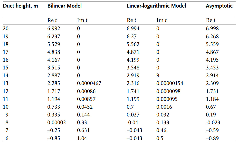
The linear-logarithmic M-profile corresponds to the case of stable stratification when the value of the M-deficit ΔM and the duct height Z_s are related via the approximate expression: ΔM = g_sZ_s, where g_s = 0,3 N-units m^–1.

The value of the M-deficit can be determined by approximating the logarithmic M-profile in the interval 0 < z < Z_s by a linear M-profile with gradient equal to

M^{'} {(z)}_{z = z_{r}},

i. e., at the sea roughness level.

As can be seen from comparison of the results in Table 4.1, for very strong M-inversion, when the mode is deeply trapped inside the duct, i. e., Re ≫ t_n ≫ 1, the propagation constants for the linear-logarithmic and bilinear profiles and asymptotical values are practically equal to each other and to asymptotical values for the linear profile:

t_{1}^{0} = μ_{1}^{3} H_{s} - μ_{1}^{2} 2, 338,

where:

μ_{1}^{3} = a \cdot 10^{- 6} g_{s} .

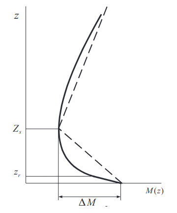
In the case of weak trapping, when Re t_n ≤ 1, the difference between the two profiles becomes significant. This is caused by the behavior of the reflection of trapped waves from a potential barrier in the vicinity of the minimum of U(h). In particular, the imaginary part of the propagation constant of the linear-logarithmic profile is less than one obtained from a linear profile since the thickness of the potential barrier is greater in the case of the logarithmic profile, Figure 2.

Fig. 2 Smooth M-profile

The contribution of the first mode in Eq. (2) in the case of the linear-logarith- mic profile can be written in a form similar to Eqs. (3) to (15):

With

H_{s} ≪ μ_{2}^{2} {|t_{1}|}^{1 / 4},

then for all h, h₀:

F_{1} (h, h_{0}) = \frac{1}{4 μ_{2}^{2} \sqrt{ξ_{1}}} e x p [j S (h, t_{1}) + j S (h_{0}, t_{1}) + j \frac{π}{3}] . E q . 19

When h, h₀ ≤ H_s:

F_{1} (h, h_{0}) = - \frac{2 D}{Λ} \sin [S (h, t_{1})] \sin [S (h_{0}, t_{1})] E q . 20

where:

D = {[(U (h) - t_{1}) \cdot (U (h_{0}) - t_{1})]}^{- 1 / 4}, Λ = 2 \frac{\sqrt{U_{0} - t_{1}}}{μ_{1}^{3}} .

When both antennas are located above the duct, i. e., h, h₀ > H_s, then:

F_{1} (h, h_{0}) = \frac{T \cdot D}{2 Λ} e x p [j S (h, t_{1}) + j S (h_{0}, t_{1})] E q . 21

where:

T = 1 - {|R_{s} (t_{1})|}^{2}, R_{s} = \frac{1}{1 + e^{2 π ν t_{1}}} . E q . 22

And, finally, when only one antenna is placed above the duct, say h > H_s, we obtain:

F_{1} (h, h_{0}) = j \frac{D}{2 Λ} \sin [S (h_{0}, t_{1})] e x p [j S (h, t_{1})] . E q . 23

In the case of an arbitrary M-profile and a finite value of the surface impedance, the solution to Eq. (1) can be found by using numerical methods. In this case we may introduce a normalised height gain function f instead of the function χ⁺(h, t):

f (h, t) = \frac{χ^{+} (h, t)}{χ^{+} (0, t)} . E q . 24

Function f is then governed by the uniform equation:

\frac{d^{2} f}{d h^{2}} + [U (h) - t] f = 0 E q . 25

and satisfies the following boundary conditions at h = 0:

f (0, t) = 1, {\frac{d f}{d h}}_{h = 0} = q E q . 26

where

q = j m / \sqrt{η} .

Note that for horizontal polarization the parameter q should be replaced by

q^{'} = j m / \sqrt{η} .

At the upper boundary of the duct, at some height h_o, h_o ≥ H_s, the function f should satisfy the condition of the outgoing wave, i. e., d/dh arg(f(h, t)) > 0. While this height can be arbitrarily chosen, in practice the profile U(h) is approximated by a linear one, thus allowing one to represent the outgoing wave via the Airy function w₁.

Equation (25) for the height-gain function f can be integrated by standard numerical methods making use of boundary conditions (26) and the analytical transition of the function and its derivative at the height h_o. The application of boundary conditions at both boundaries h = 0 and h = h_o leads to the characteristic equation Q(t_n) = 0 for the propagation constants t_n.

The attenuation factor W in the shadow region can then be represented as the sum of normal waves equivalent to the residue sum of the integral (Wave Field Fluctuations in Random Media over a Boundary Interfacein this equation) in the poles of the S-matrix:

W (ξ, h, h^{'}) = 2 e^{j π / 4} \sqrt{π ξ} \sum_{n = 1}^{\infty} e^{j ξ t_{n}} \frac{d t_{n}}{d q} f (h, t_{n}) f (h^{'}, t_{n}) E q . 27

where parameter:

\frac{d t_{n}}{d q} = - {[\frac{d}{d h} {(\frac{\partial f}{\partial t_{n}})}_{h = 0}]}^{- 1}

is called the excitation coefficient of the normal wave with number n.

The characteristic equation Q(t_n) = 0 in the general case can be realised in computer-based calculations by simultaneously solving Eq. (25) for height-gain functions with a trial value of t_n. In the case of the bilinear profile (2) the characteristic equation Q(t_n) = 0 is exactly the same as Eq. (3).

In the case of the linear-logarithmic profile, as shown in UHF Propagation in an Evaporation Duct“Some Results of Propagation Measurements and Comparison with Theory”, the refractivity profile close to the sea surface can be replaced at the heights h < h_r by a linear segment with appropriate gradient without appreciable errors in the estimation of the propagation constant. In that case the resulting profile consists of three segments:

the linear profile in the interval 0 ≤ h < h_r,;
the logarithmic profile U(h) = U(h_r)-κ ln (η/h_r);
and the linear profile at heights h > h_o.

In this case the solution to Eq. (8) should be tailored in terms of the continuity of the function f and its derivative df/dh with analytical representa- tion of the function f via Airy functions in linear segments.

The numerical algorithm for finding the propagation constants can be implemented in the following way. Assume that we know the etalon solutions

t_{n}^{0}

for a specific profile U₀(h). The respective characteristic equation we denote as

Q (t_{n}^{0}) .

. Instead of the equation Q(t_n) = 0 for the propagation constant of the problem we may use:

Q (t_{n}, σ) = (1 - σ) Q (t_{n}^{0}) E q . 28

introducing a new parameter σ varying between 0 and 1. The roots of Eq. (28) depend on thevalue of σ. When σ = 0 we have a solution of the etalon problem, i. e.

t_{n} = t_{n}^{0},

, with σ = 1 the solution to Eq. (28) gives “true” propagation constants. With variation in σ from 0 to 1 the roots of Eq. (28) traverse along some trajectories in the complex plane t from

t_{n}^{0}

to t_n. The equation for the trajectories is:

\frac{d t_{n}}{d σ} = - \frac{Q (t_{n}^{0})}{\frac{\partial}{\partial t_{n}} Q (t_{n}, σ)} . E q . 29

In practice, the parameter σ should be related to one of the inherent parameters of the problem, i. e., this might be the impedance q, the height of the duct H_s or the gradient of the M-profile above or below H_s. In that case the trajectories of the roots t_n(σ) are likely to be restrained by their own valley in the module profile of |Q(t_n, σ)| in the plane of complex t.

The algorithm based on the evolution of the height of the evaporation duct has been implemented in a radio coverage prediction system with the close participation of the author. In that system we used a bilinear approximation of the linear-logarithmic M-profile for the evaporation duct described in terms of a single parameter, the height of the duct, H_s. The approximating linear profile reveals an almost constant gradient within h < H_s thus allowing one to use one parameter H_s to build the evolution algorithm similar to Eq. (11) and create look-up tables for pre-calculated propagation constants t_n(H_s).

Various well-developed methods of calculation of the propagation constants can be found in the literature. The formalism of the duct propagation in a stratified troposphere has been developed in a number of classical works started in the 1940s. Until now, those publications provide a benchmark reference and a framework for the detailed study of duct propagation. The practical algorithms incorporating the mode theory have been implemented in various computer-based programs and prediction systems. Among known models of the M-profile describing the average refractivity in the atmospheric boundary layer, the linear-logarithmic profile is accepted as the most adequate M-profile model for the evaporation duct to be utilised in development of the radar coverage prediction systems.

Author

Olga Nesvetailova

Freelancer

Literature

Jensen, N.O., Lenshow, D.H. An observational investigation on penetrative convection. J.Atmos.Sci., 1978, 35(10), 1924–1933.;
Monin, A.S., Yaglom, A.M. Statistical Fluid Mechanics, Vol.1, MIT Press, Cambridge, MA, 1971, p. 769.;
Gossard, E.E. Clear weather meteorological effects on propagations at frequencies above 1 GHz, Radio Sci., 1981,16(5), 589–608.;
Tatarskii, V.I. The Effects of Turbulent Atmo- sphere on Wave Propagation, IPST, Jerusalem, 1971.;
Gavrilov, A.S., Ponomareva, S.M. Turbulence Structure in the Ground Level Layer of the Atmosphere. Collected Data, Meteorology Series, No.1, Research Institute for Meteorological Information, Obninsk (in Russian), 1984.;
Kukushkin, A.V., Freilikher, V.D. and Fuks, I.M. Over-the-horizon propagation of UHF radio waves above the sea , Radiophys. Quantum Electron. (translated from Russian), Consultant Bureau, New York , RPQEAC 30 (7), 1987, 597–620.;

Footnotes