The simulation of the manoeuvres are conducted in Vessel Simulator (VeSim). VeSim uses two different input plug-ins and requires additional information on propulsive units and environment. The plug-in tools are HullVisc and VeRes, which calculates the hydrodynamic properties, as well as the transfer functions for the vessel motions and loads in the frequency domain, respectively.
For an overview of the structure of VeSim see Basic Ship Motions and Mathematical Model used in Vessel Simulator (VeSim) Tool“Flowchart of VeSim structure”.
The hydrodynamic coefficients calculated by HullVisc can be of questionable validity. This is because of the method used by HullVisc for calculations is a regression analysis of benchmarking vessels. The benchmark vessels are of older design and not in the same category as MF Landegode.
The simulated manoeuvres should ideally have the same environmental conditions as the full-scale trials. As the simulated manoeuvres are carried out using the “Calm water manoeuvring” option of the Vessel Simulator, there will not be a 100 % similarity between the simulated and the full-scale manoeuvres. This is because the wind, current and wave forces are excluded in this model. A certain grade of deviation is therefore to be expected.
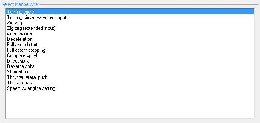
The simulated manoeuvres are the turning circle manoeuvre, the zig-zag manoeuvre, an altered version of the full astern stopping manoeuvre, the thruster turning manoeuvre (thruster twist manoeuvre) and the accelerating turn manoeuvre. Picture 1 presents a list over the different calm water manoeuvres executable in VeSim.
The main parameters needed for the propulsion input are:
- Propeller x, y and z position;
- Propeller diameter, pitch and blade area;
- Rudder height, root chord and total area;
- Wake fraction and thrust deduction;
- Engine-propeller gear ration and mechanical efficiency;
- Engine MCR, RPM and moment of inertia.
The vessel geometry used for the simulations is an adopted model developed by MARINTEK. The vessel lines and principal characteristics are pre-defined in this geometry model. The loading condition for the designed waterline is set to:
where:
- T – is the vessel’s draught.
Additionally, the operational condition, with a midship draught of Tm = 3, 60 m and a trim in the fore part of +0,752 m resulting in a fore part draught of TFP = 2, 848 m and an aft part draught of TAP = 4, 352 m, is pre-defined. The bow thrusters and the aft thruster are only taken into account when the thruster turning (thruster twist) and the accelerating turn manoeuvre are simulated.
Nomenclature for all the formulas you can see here: Nomenclature and Greek Symbols
Every manoeuvre is simulated with the operational draught and trim described above.
Results from VeSim
The following sections present the results obtained from the simulations and present them in form of tables and a brief discussion. The tables will give a comparison of the simulated manoeuvres with the IMO requirements as in the full-scale trials. As the vessel geometry model is symmetric about the centreline, it was expected the results would be identical to port and starboard, this was however not the case. The different tables will list results of both starboard and port manoeuvres.
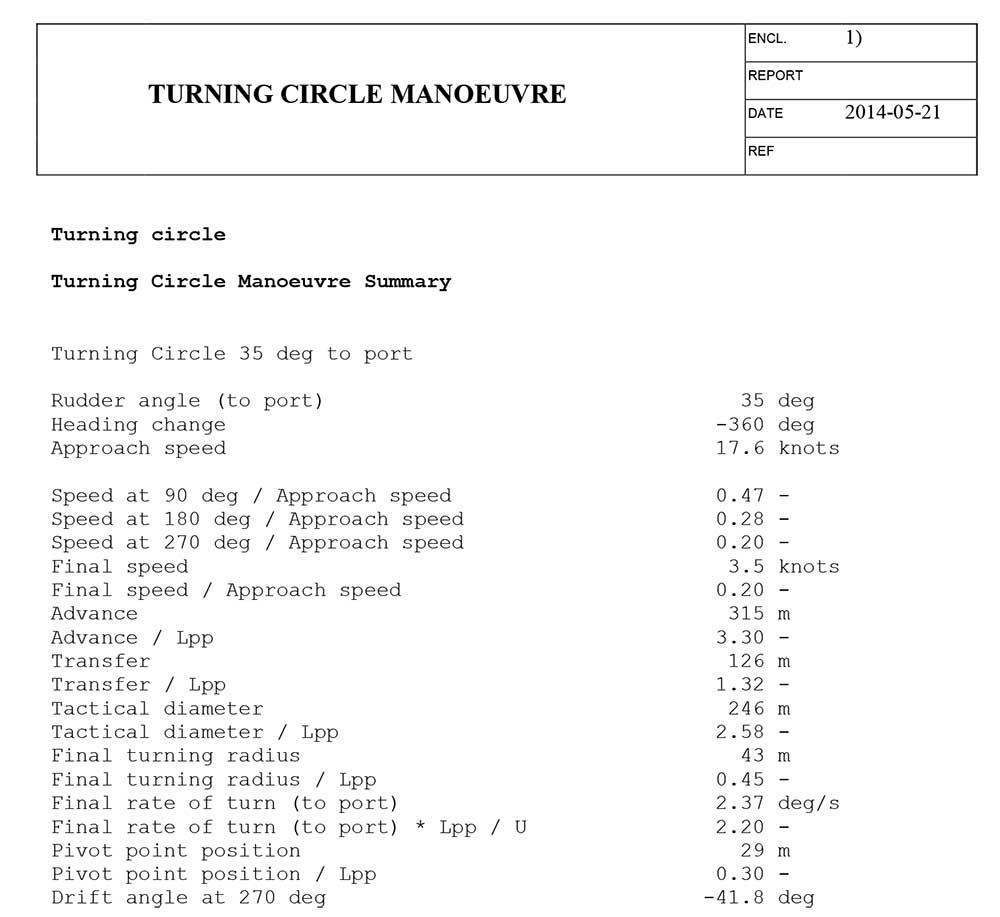
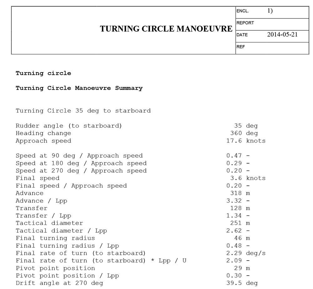
Turning circle manoeuvre
When simulating the turning circle, the user must set the desired initial vessel speed, maximum heading (i. e. the heading when the test is accomplished), the rudder angle to be used, if the manoeuvre is to starboard or port, and whether or not to include a pull-out test and its duration.
When evaluating the results of the simulated turning circle manoeuvre, one should have in mind that the simulation is conducted without changing the pitch and RPM of the propeller, which was the case for the full-scale manoeuvre. Some differences between the full-scale and simulated manoeuvres are hence expected.
The results of the simulation is shown in the table below.
| Table 1. Simulated turning circle results | ||||
|---|---|---|---|---|
| Port | Starboard | IMO | ||
| Tactical diameter | [m] | 246 | 251 | 450 |
| Transfer | [m] | 126 | 128 | – |
| Advance | [m] | 315 | 318 | 405 |
| Rudder angle | [°] | 35 | -35 | – |
| Approach speed | [kn] | 17,6 | 17,6 | – |
| Final speed | [kn] | 3,5 | 3,6 | – |
From Table 1 showing the the simulated turning circle manoeuvre, the results are well within the IMO requirements.
Regarding the simulated results, they appear to be of genuine validity with some discrepancy from the full-scale results in Simulation of the Full-Scale Sea Trials from the Marine Activities and Offshore Operations Project“Full-scale port turning circle results”.
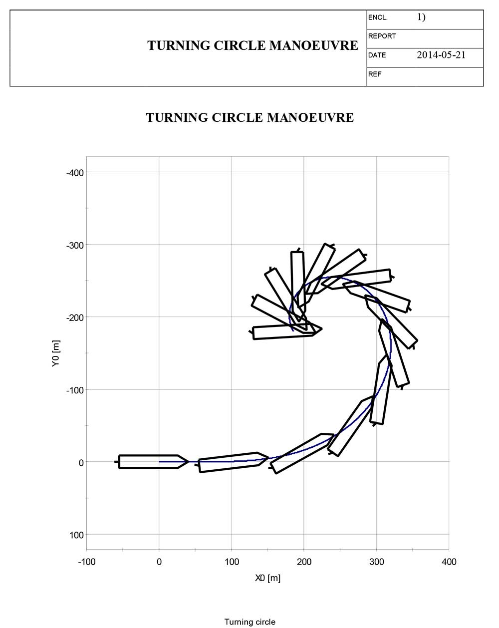
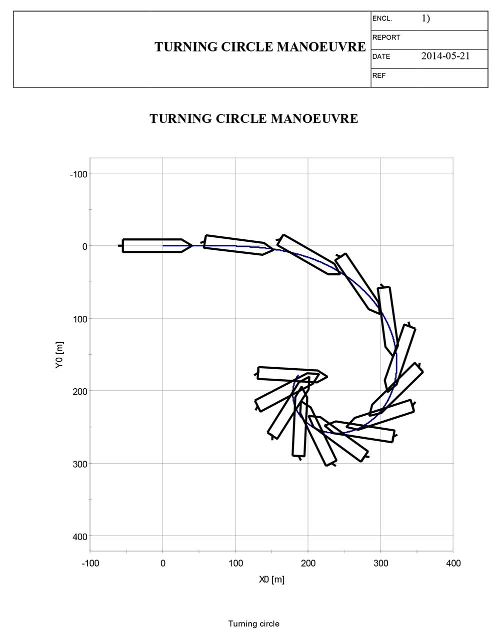
But if the trajectory plot of the simulated manoeuvre is interpreted, one can clearly observe the inequality between the full-scale and simulated manoeuvre. This also confirms the inadequate quality of the coefficients calculated by HullVisc.
The simulated trajectory plot is shown on pictures below.
VeSim simulated manoeuvres
Starboard turning circle
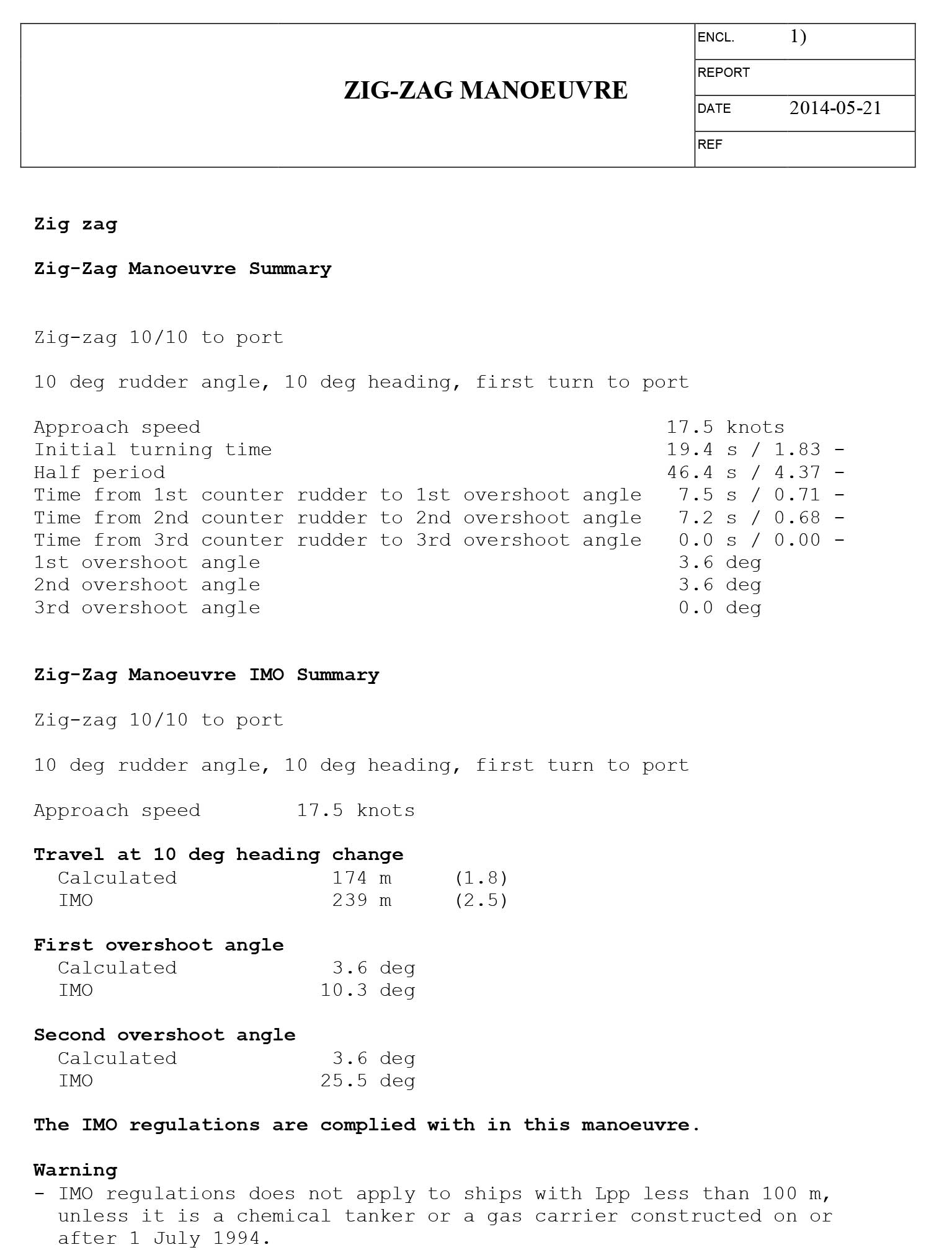
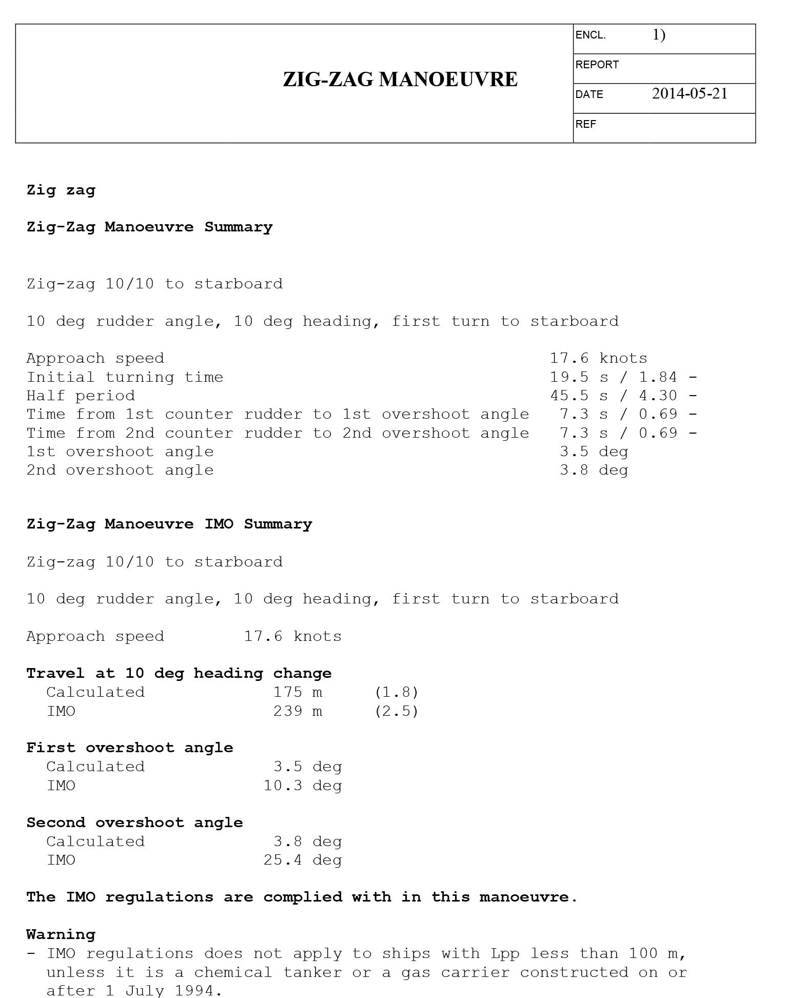
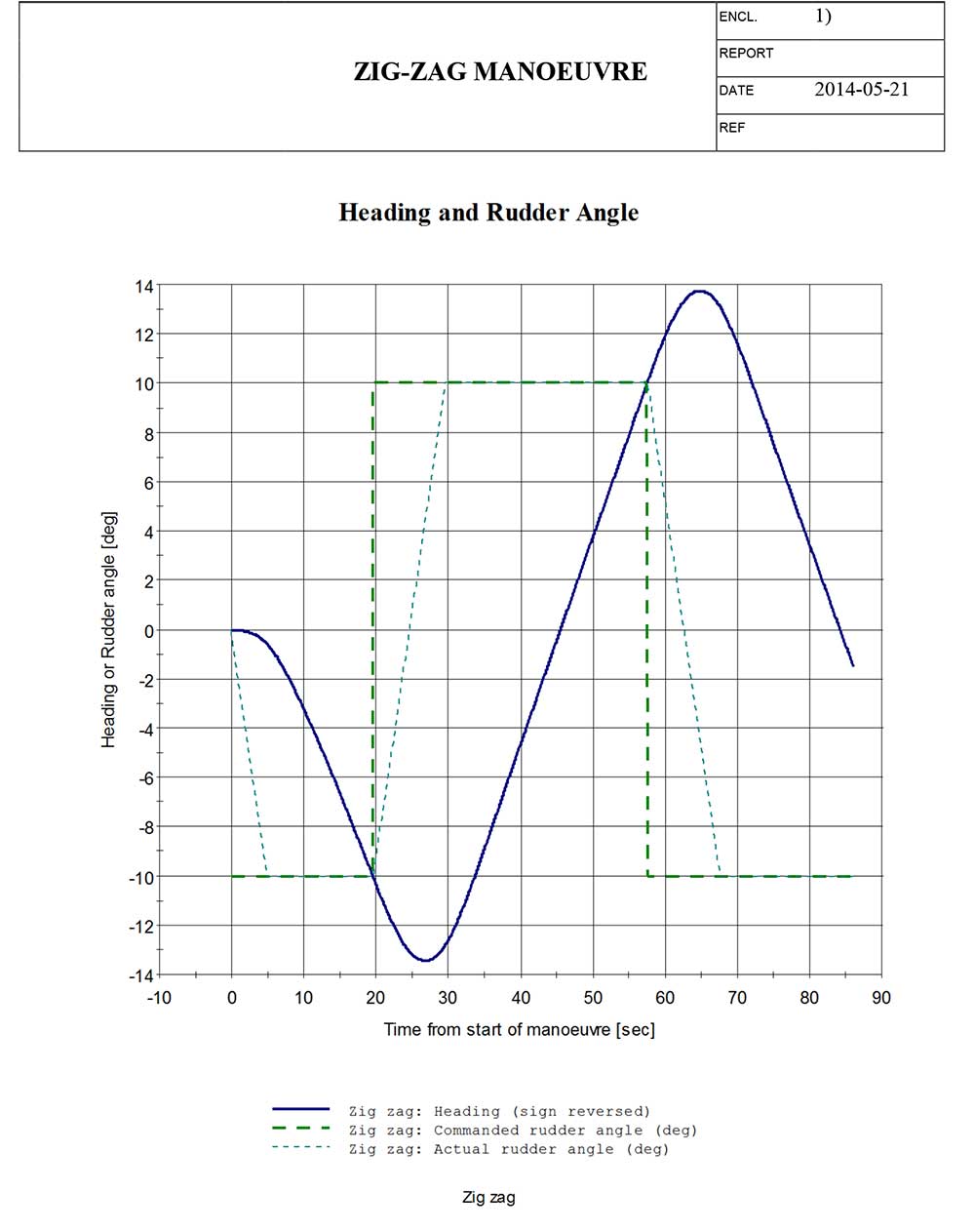
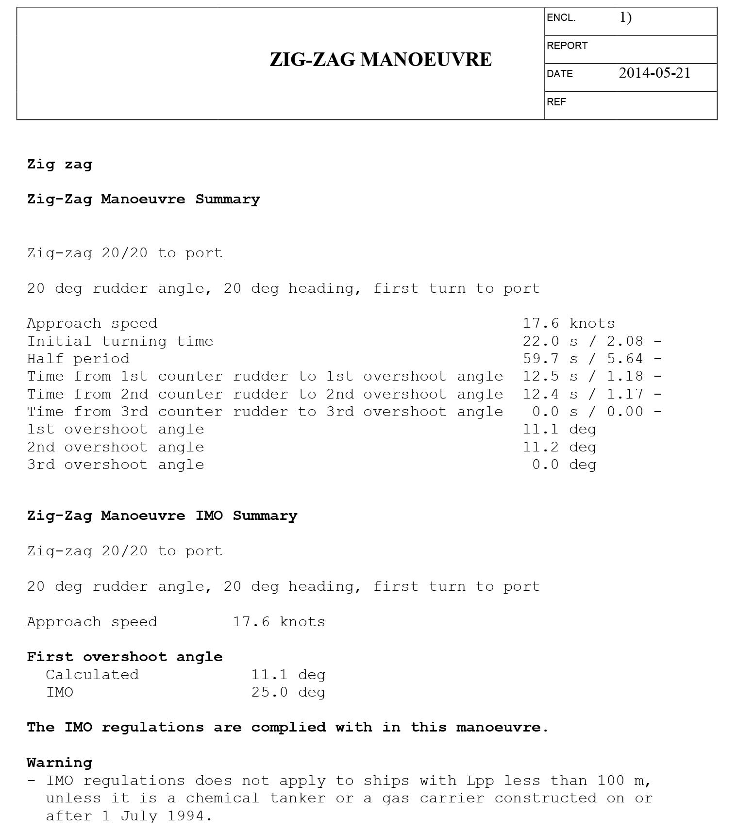
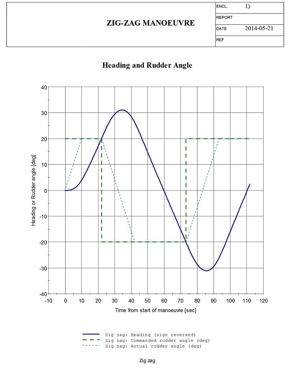
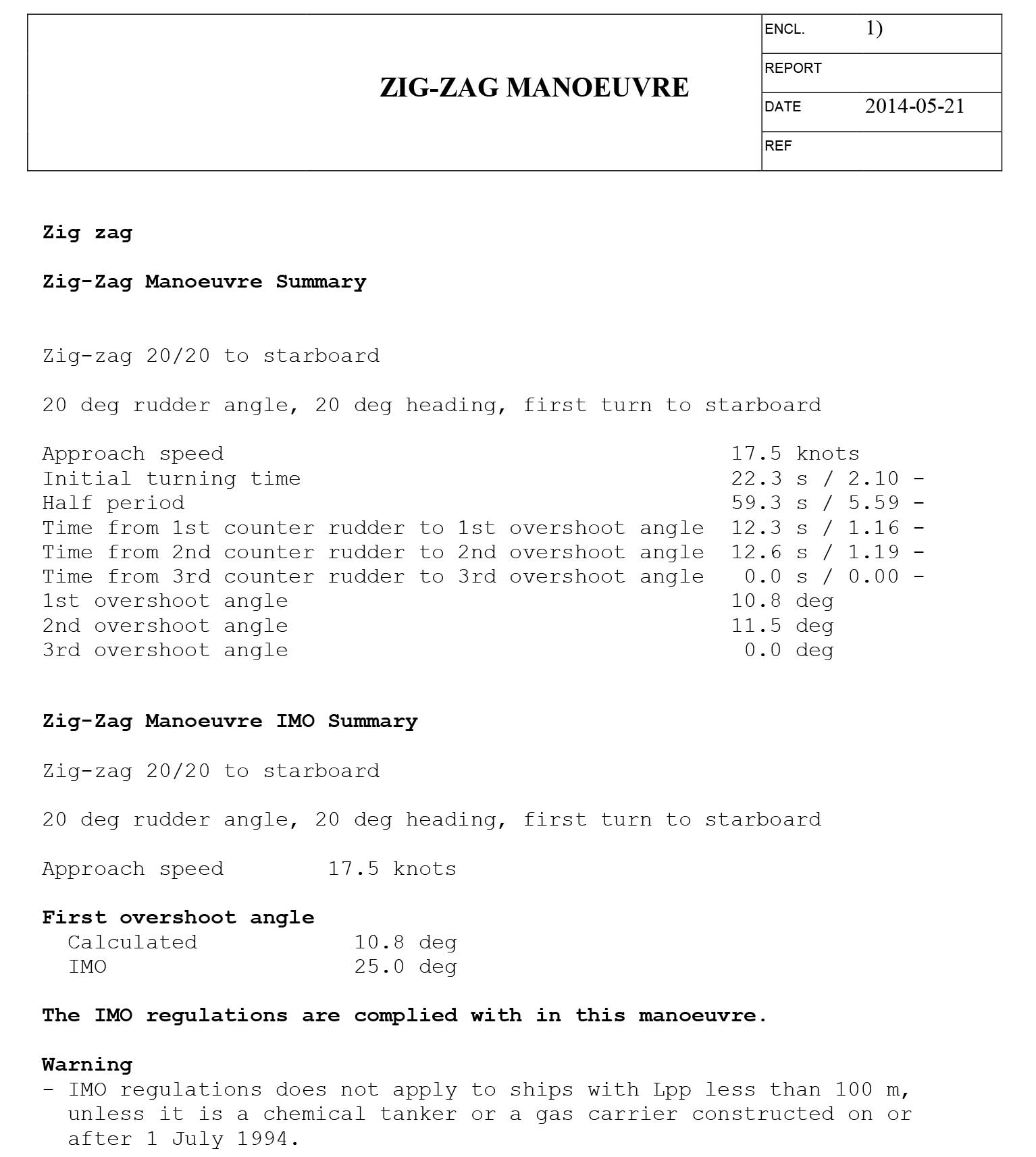
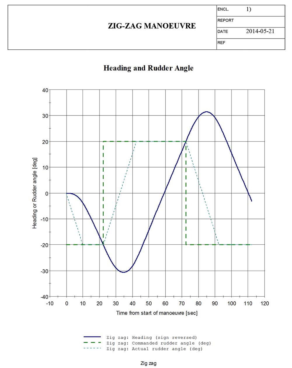
Zig-zag manoeuvre
The parameter input needed in the zig-zag manoeuvre are the initial vessel speed, the commanded rudder angle, the heading change achieved before rudder change and the number of overshoot angles to be calculated.
The result of the simulations are shown in the following Table 2.
| Table 2. Simulated 10/10 and 20/20 zig-zag results | |||||||
|---|---|---|---|---|---|---|---|
| Port | Starboard | IMO | |||||
| 10/10 | 20/20 | 10/10 | 20/20 | 10/10 | 20/20 | ||
| Approach speed | [kn] | 17,5 | 17,6 | 17,6 | 17,6 | – | – |
| Time from 1st counter rudder to 1st overshoot angle | [s] | 7,5 | 12,5 | 7,3 | 12,5 | – | – |
| Time from 2nd counter rudder to 2nd overshoot angle | [s] | 7,2 | 12,4 | 7,3 | 12,4 | – | – |
| 1st overshoot angle | [°] | 3,6 | 11,1 | 3,5 | 10,8 | 10,0 | 25,0 |
| 2nd overshoot angle | [°] | 3,6 | 11,2 | 3,8 | 11,5 | 25,0 | – |
Table 2 giving the result of the zig-zag manoeuvre indicates that the simulated manoeuvre is of desirable validity and well within the IMO requirements for both the 10/10 and the 20/20 manoeuvre.
The main results and plots of the simulation is presented below.
Zig-zag manoeuvre
Port 10/10 zig-zag manoeuvre

Starboard 10/10 zig-zag manoeuvre
Port 20/20 zig-zag manoeuvre
Starboard 20/20 zig-zag manoeuvre
Stopping test
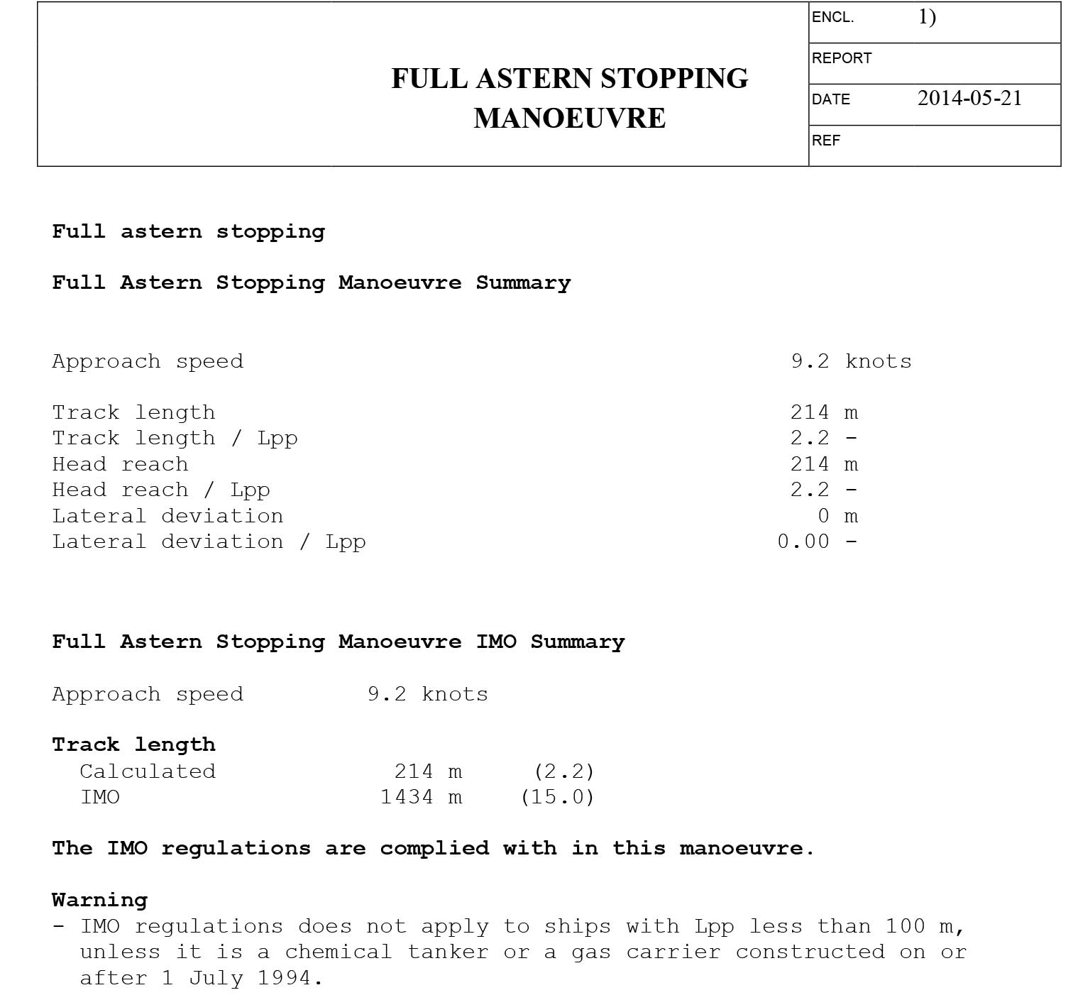
When simulating the stopping manoeuvre, named “Full astern stopping” in Basic Ship Motions and Mathematical Model used in Vessel Simulator (VeSim) ToolVeSim, the user needs to determine the initial vessel speed and the commanded engine setting astern. The simulator does not give the user the possibility of altering the pitch of the propeller instead of reversing the engine. When evaluating this manoeuvre and comparing to the full-scale test, one need to bear in mind the different approach methods used for this manoeuvre, i.e. the use of reverse engine and propeller pitch. With this in mind, the results of the simulation are shown in the following Table 3.
| Table 3. Simulated stopping test results | ||
|---|---|---|
| VeSim simulation | ||
| Track length | [m] | 214 |
| Ship length | [-] | 2,4 |
Table 3 lists the result of the simulated stopping manoeuvre. The results are not compared with the IMO requirements as the manoeuvre is not performed with a maximum approach speed as described in the IMO MSC/Circ. 1053, but with an approach speed of 9,2 knots, as in the full-scale manoeuvre.
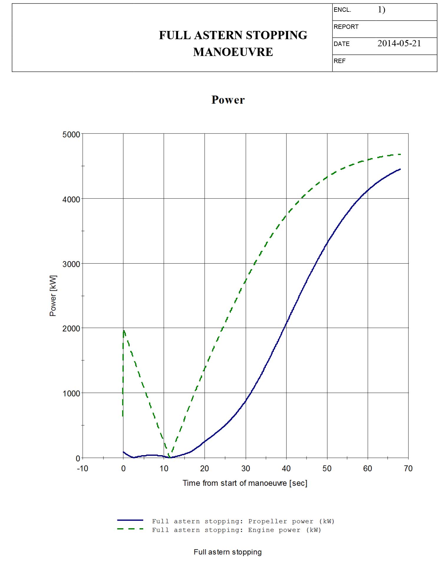
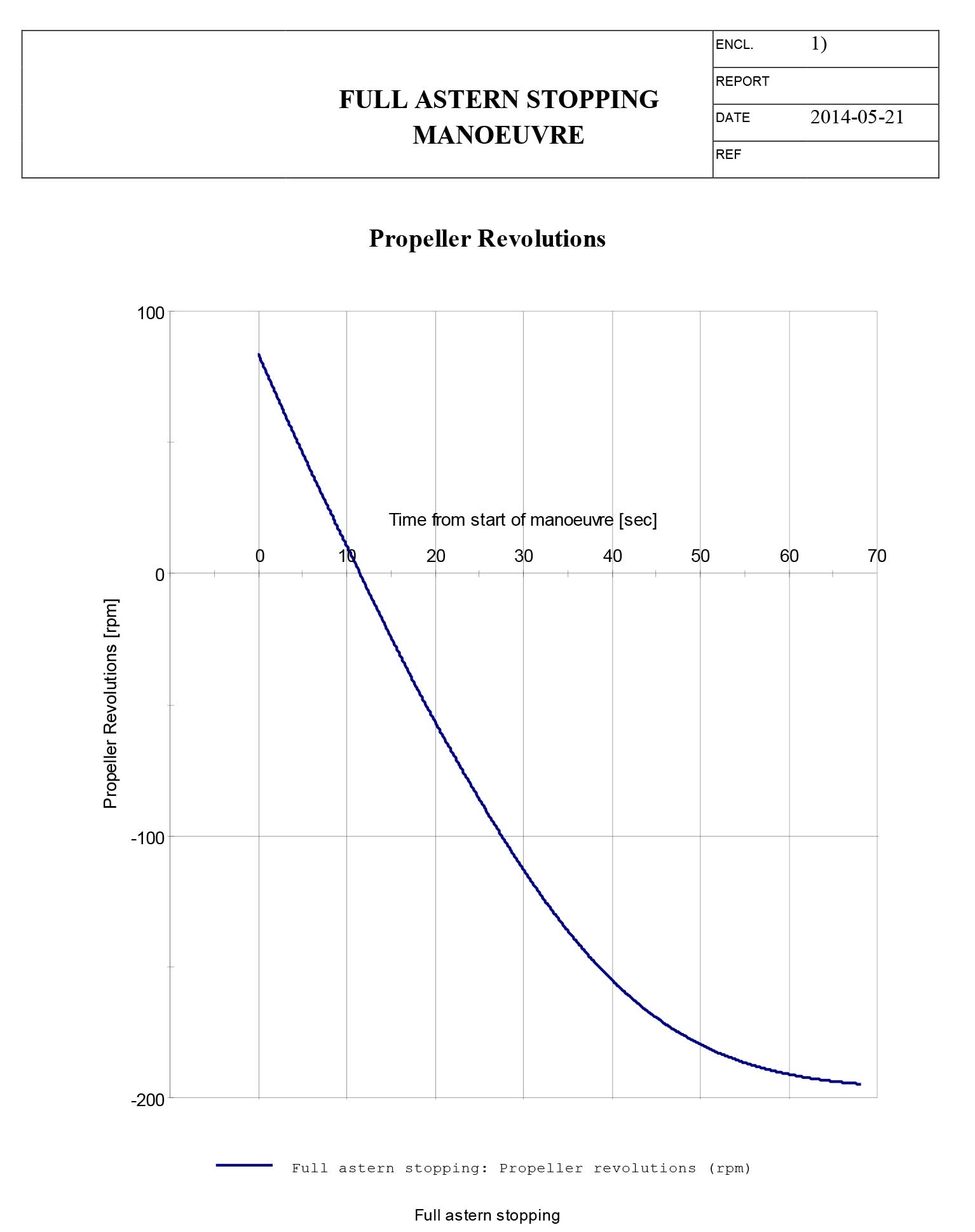
The main results and plots of the simulation are presented in below.
Full astern stopping manoeuvre – results
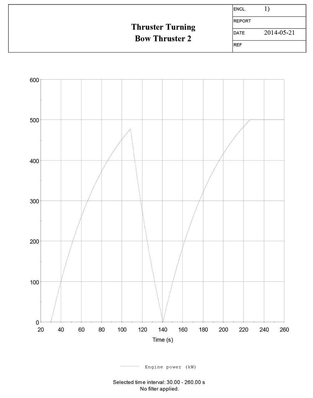
Thruster turning manoeuvre
The thruster turning manoeuvre, as described in the “International Standard ISO 13643-2″, is not a standard manoeuvre in the list of executable manoeuvres in VeSim. However, a similar manoeuvre called “Thruster twist” is available, but this manoeuvre will only rotate the vessel about its own axis in a continuously directional motion by use of thrusters, until the end of the time sequence is reached.
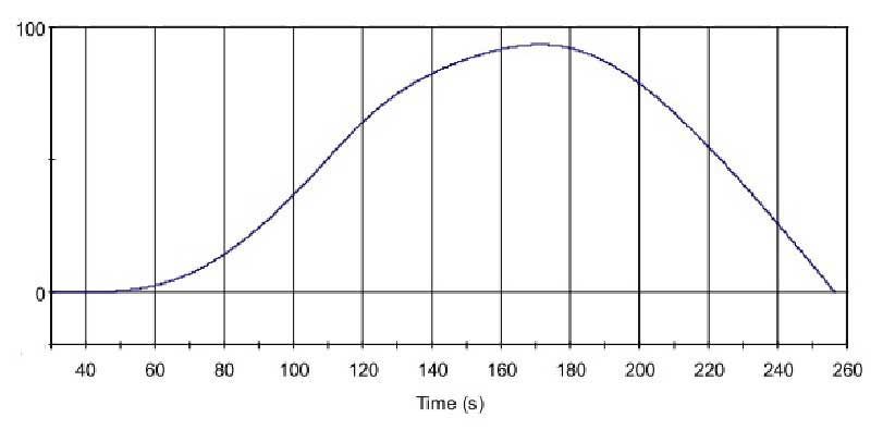
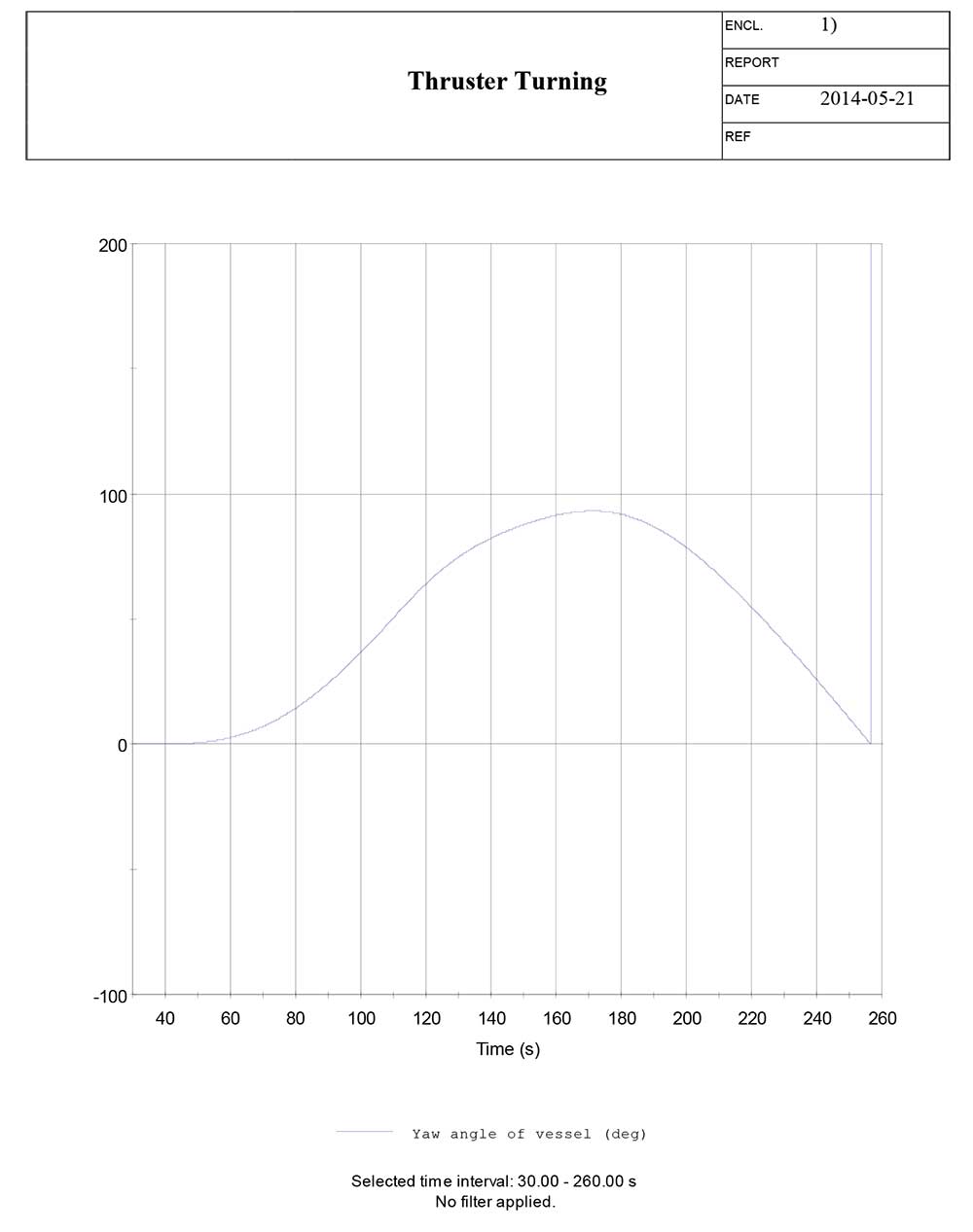
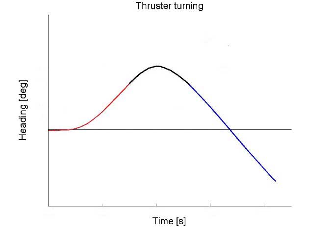
To simulate the thruster Information about Vessel Manoeuvring based on IMO Standardsturning manoeuvre, the manoeuvre must be manually commanded in the time domain simulator. By doing so, the thrusters are commanded to 100 % by the command “Tunnel_Thruster1_Actuator cmd_revs 100.0” in the scenario manager tab, as illustrated in Picture 2. The time of the thruster executions are found by evaluating the yaw angle [deg] from the thruster twist manoeuvre.
The time needed to reach a 60° heading change is logged from the thruster twist and used in the time domain simulation to give the command to reverse the thrusters. By plotting the yaw angle versus time, the time needed for reaching a heading of 15, 30, 60, maximum, return to 60, return to 30 and return to 0 degrees can be obtained, including the overshoot angle and time.
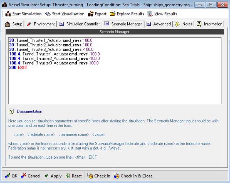
Table 4 lists the results obtained from the manual time domain simulation. Picture 3 depicts the heading of the vessel and the time steps corresponding to Table 4. The time of manoeuvre execute in Picture 3 is at t = 30 sec.
| Table 4. Simulated thruster turning results | ||
|---|---|---|
| VeSim simulation | ||
| t15 | [s] | 30,3 |
| t30 | [s] | 42 |
| t60 | [s] | 62,4 |
| ts | [s] | 87,9 |
| t60R | [s] | 116,4 |
| t30R | [s] | 136,6 |
| t0R | [s] | 154,9 |
| ∆ts | [s] | 25,5 |
| ψs | [deg] | 82,52 |
| ∆ψs | [deg] | 22,52 |
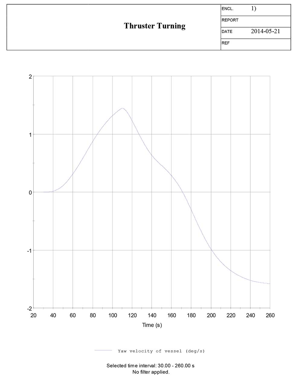
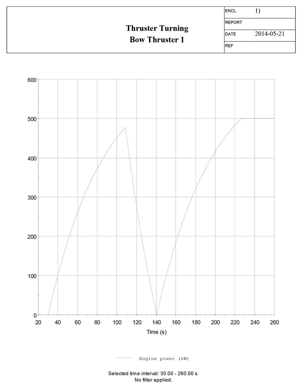
The main results and plots of the simulated manoeuvre is presented below.
Thruster turning manoeuvre – results

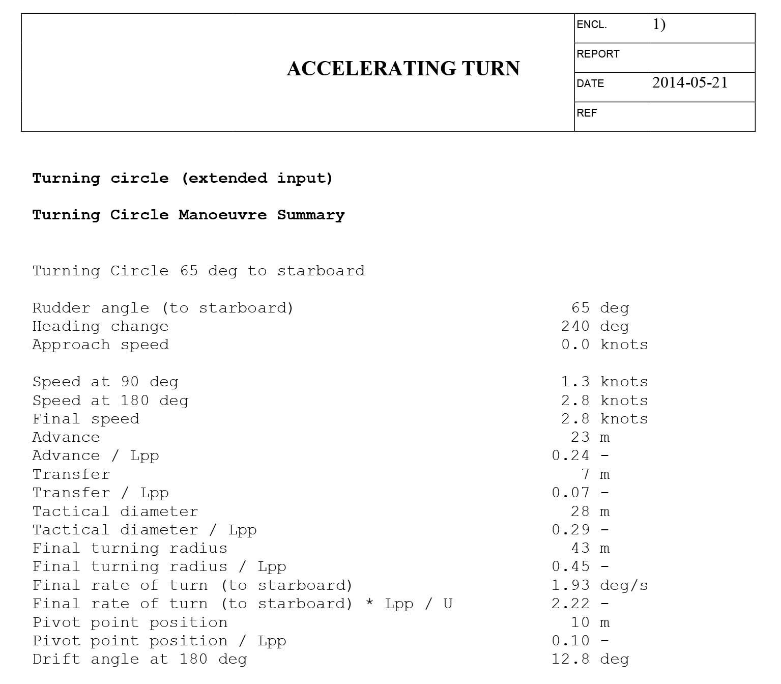
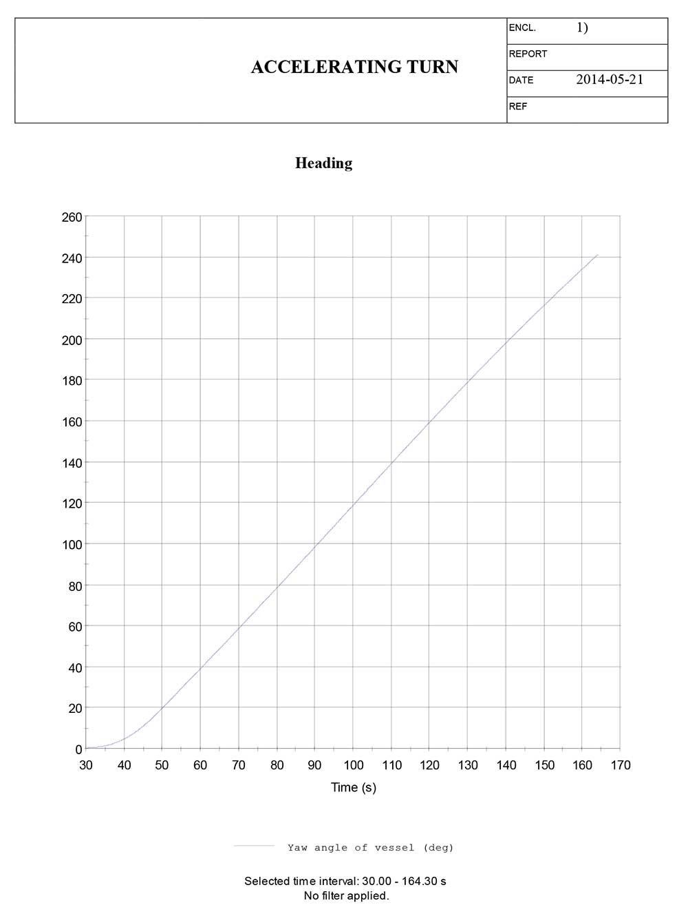
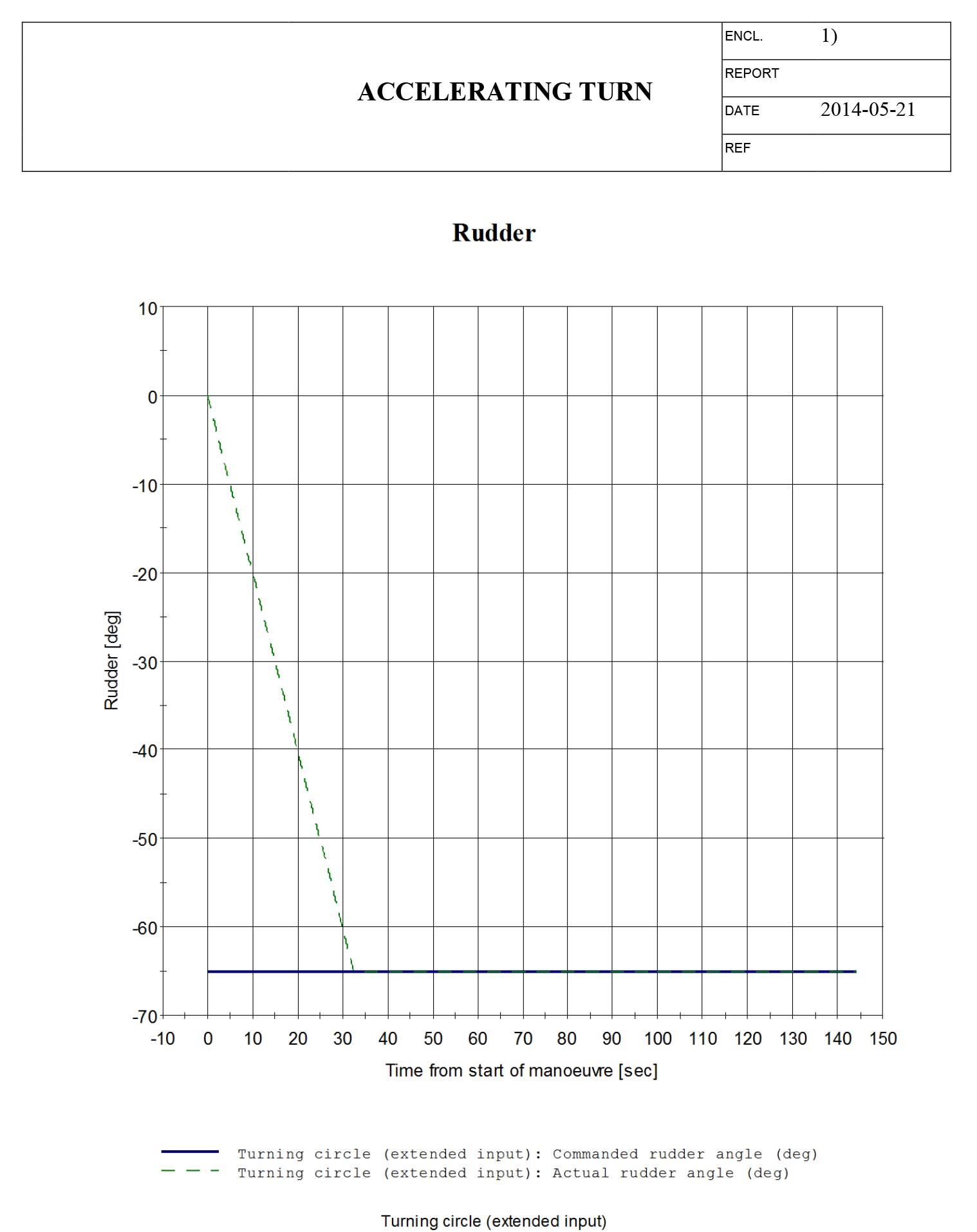
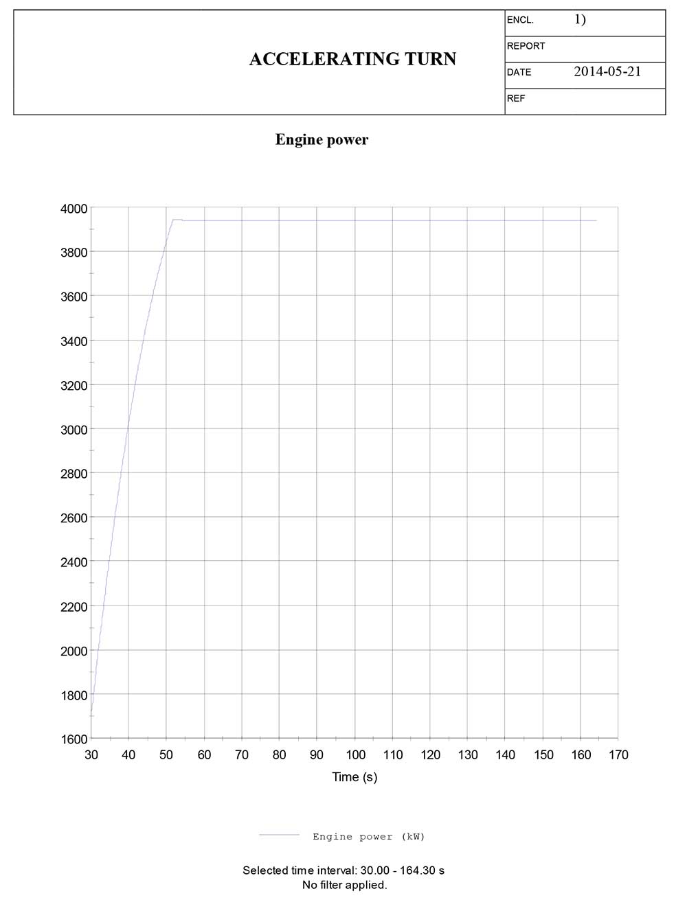
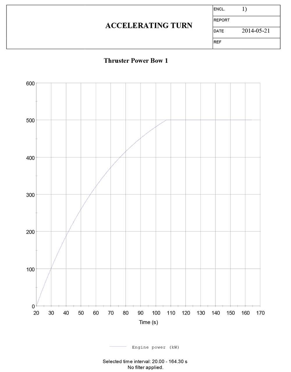
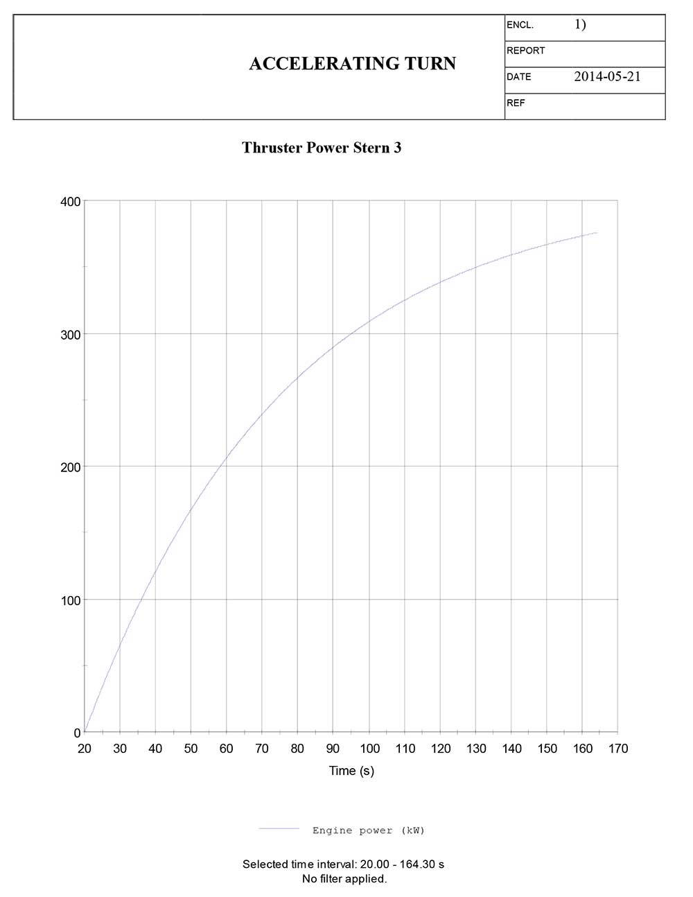
Accelerating turn manoeuvre
The accelerating turn manoeuvre is also not a basic manoeuvre from the selected list of executable manoeuvres. But the “Turning circle (extended input)” manoeuvre allows the user to provide input for multiple parameters that is not included in the basic turning circle manoeuvre input. E. i. the use of thruster power. The advance, transfer and tactical diameter are given by the standard output in the ShipX plot, but the speed at-, and the time to turn 90° and 180° are found by manually plotting the yaw angle [deg] and speed [m/s] versus time, and further extracting the corresponding values.
The results of the accelerating turn manoeuvre is listed in Table 5 below.
| Table 5. Simulated accelerating turn results | ||
|---|---|---|
| VeSim simulation | ||
| Advance | [m] | 23 |
| Transfer | [m] | 7,0 |
| Tactical diameter | [m] | 28 |
| Time to turn 90° | [s] | 65,9 |
| Time to turn 180° | [s] | 110,7 |
| Speed at 90° change of heading | [kn] | 1,07 |
| Speed at 180° change of heading | [kn] | 2,74 |
The main results and plots of the simulated manoeuvre is presented below.
Accelerating turn manoeuvre – results

Comparison of simulated and full-scale results
Here, a comparison of the simulated and full-scale manoeuvring trials will be presented as a set of different graphs, most with a best fit trend line. Different combinations of colour and markers are used to indicate the different characteristic measurements of the manoeuvre currently analysed. These marker and colour combinations are listed in the corresponding table for each manoeuvre. The different graphs are a graphical presentation of the full-scale and simulated results.
From the different graphs a clear observation can be made on whether the simulations are over- or underestimated. As the graphs indicate, most of the simulated results are overestimated. This can be a result of the underestimated hydrodynamic coefficients calculated by HullVisc. Other error sources in predicting the manoeuvres may be from the mathematical model used in VeSim and VeRes, as viscous effect, cross flow drag, propeller, rudder and thruster forces.
Turning circle manoeuvre
| Table 6. Markers for comparison of simulated and full-scale turning circle results | ||||||
|---|---|---|---|---|---|---|
| Original | Corrected | |||||
| Advance | Transfer | Tactical | Advance | Transfer | Tactical | |
| Port | Red * | Cyan * | Blue * | Black * | Magenta * | Green * |
| Starboard | Red o | Cyan o | Blue o | Black o | Magenta o | Green o |
Picture 4 depicts the simulated and full-scale turning circle manoeuvre. Both the original full-scale results and the current corrected results are plotted in the picture. The linear blue line indicates the best fit trend line where the results from simulations and full-scale would be similar. Table 6 explains the different marker and colour combinations used in Picture 4, where “original” and “corrected” refers to the current correction.
From Picture 4 it can be observed a clear tendency of overestimation of the simulated manoeuvres. Only the port tactical diameter is underestimated, but however fairly close to the full-scale trial result. As is the starboard tactical diameter, both presented as listed in Table 6. The Advance and transfer is overestimated in a large extent as they are not very close to the best fit line. The fact that the different calculations have a different percentage of error margin may indicate an unstable simulation of the manoeuvre. This is mainly concerning the calculation of advance, since this parameter is the one farthest away from what was the desired outcome.
Zig-zag manoeuvre
In Picture 5 the different overshoot angles are plotted for each rudder angle in both the port (positive values) and starboard (negative values) direction. The circle markers indicate simulated manoeuvres, the x markers indicate full-scale manoeuvres, whereas the red and blue colour represent the first and second overshoot angle, respectively. The results are as listed in table Simulation of the Full-Scale Sea Trials from the Marine Activities and Offshore Operations Project“Full-scale zig-zag results” and 2 for the full-scale and simulated manoeuvres, respectively.
Picture 5 give an impression of the similarity between the 10/10 and 20/20 manoeuvre, and the 1st and 2nd overshoot angle to both starboard and port.

As the picture illustrates, there is a high rate of compliance between the simulated starboard and port manoeuvre, for both the 10/10 and the 20/20 rudder angle. The full-scale measurements show a fair rate of compliance, but with a segregate in the 10/10 port 2nd overshoot angle, as it is larger than the 1st overshoot angle which contradicts the tendency of the other full-scale results. This may be an error in the specific run and should be evaluated with care. The picture also illustrates the similarity between the 1st and 2nd overshoot angle in the simulated manoeuvre, as they are almost identical, unlike the full-scale results.
Read also: Introduction to the Standard Simulation Tests and Requirements for Naval Hydrodynamics
In Picture 6 the same results are plotted, but as a best fit trend line between the simulation and full-scale measurements. The corresponding colour and marker combinations are listed in Table 7. As the picture illustrates, the 2nd overshoot in the 20/20 starboard and port manoeuvre is the only overestimated calculation in VeSim, whereas the other calculations are underestimated. It can also be observed that there is a tendency of underestimating the calculations with the same magnitude, as the markers are about the same proportion of magnitude below the best fit line. This indicates that there is a certain stability in the simulations, albeit they are, for the most part, underestimated.
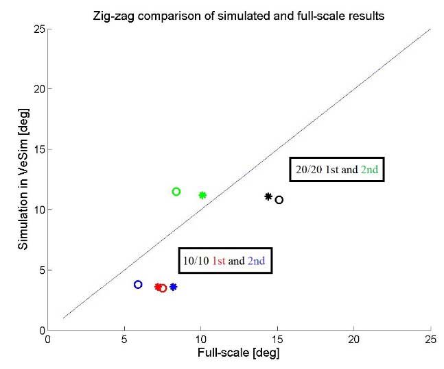
| Table 7. Markers for comparison of simulated and full-scale zig-zag results | ||||
|---|---|---|---|---|
| 10/10 | 20/20 | |||
| 1st overshoot | 2nd overshoot | 1st overshoot | 2nd overshoot | |
| Port | Red * | Blue * | Black * | Green * |
| Starboard | Red o | Blue o | Black o | Green o |
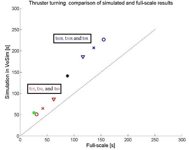
Thruster turning manoeuvre
Picture 7 depicts the different time calculations of the thruster turning manoeuvre. The full-scale and simulated results listed in tables Simulation of the Full-Scale Sea Trials from the Marine Activities and Offshore Operations Project“Full-scale thruster turning results” and 4, respectively, are plotted with marker and colour combinations as listed in Table 8.
Picture 8 is a dummy figure, intended for illustrating the use of the different colour combinations presented in Table 8.
| Table 8. Markers for comparison of simulated and full-scale thruster turning results | ||
|---|---|---|
| Marker | ||
| t15 | [s] | Red o |
| t30 | [s] | Red x |
| t60 | [s] | Red ▽ |
| ts | [s] | Black * |
| t60R | [s] | Blue ▽ |
| t30R | [s] | Blue x |
| t0R | [s] | Blue o |
| Δts | [s] | Green * |
As Picture 7 illustrates, the time simulated results are overestimated for all heading reaches. A tendency of increasing the margin of error can be observed as the different simulated heading angles are reached after increasing time steps. The simulation model is stable considering not having calculations that disperse from the trend in a large extent, but increases the time needed to obtain the desired heading reach with a constant degree of error.
Accelerating turn manoeuvre
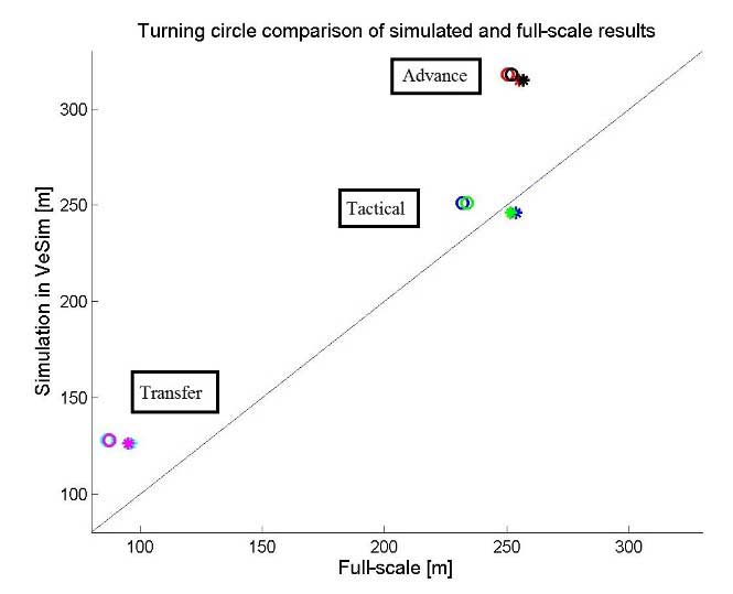
In Picture 9, the results of the full-scale and simulated accelerating turn manoeuvre, listed in tables Simulation of the Full-Scale Sea Trials from the Marine Activities and Offshore Operations Project“Full-scale accelerating turn results” and 5, respectively, are plotted in combinations of marker and colour. The different combinations are listed in Table 9. The left y-axis in Picture 9 refers to the simulations in metres and the right y-axis refers to the time in seconds. As the figure illustrates, the simulated transfer calculation is 100 % identical to the full-scale measurement, as it appears exactly on the best fit trend line.
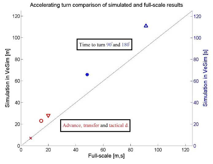
The advance and tactical diameter are however overestimated, but in the same magnitude of error, indicating a stable simulation model. This is also the case for the time to turn 90 and 180 degrees, indicated in Picture 9 as described in Table 9.
| Table 9. Markers for comparison of simulated and full-scale accelerating turn results | ||
|---|---|---|
| Marker | ||
| Advance | [m] | Red o |
| Transfer | [m] | Red x |
| Tactical diameter | [m] | Red ▽ |
| Time to turn 90° | [s] | Blue * |
| Time to turn 180° | [s] | Blue Δ |