Understanding Coherence Function in Random Atmospheres

Dive into the study of coherence function in random and non-uniform atmospheres. This article examines the approximate extraction of eigenwaves from the discrete spectrum, particularly in the context of evaporation ducts.

СодержаниеСвернуть

Approximate Extraction of the Eigenwave of the Discrete Spectrum in the Presence of an Evaporation Duct
Equations for the Coherence Function

Learn about the essential equations that define the coherence function and their significance in atmospheric research and applications. Perfect for researchers and enthusiasts in the field of atmospheric science.

Approximate Extraction of the Eigenwave of the Discrete Spectrum in the Presence of an Evaporation Duct

Consider Green Function for a Parabolic Equation in a Stratified Mediumthis equation in the case when the evaporation duct is present in the height interval (0, H_s). Let us seek a solution to the attenuation function W in the expansion over the system of eigenfunctions of the continuous spectrum defined in Understanding Parabolic Approximation in Wave Propagation: Analytical Methods and Applications“Parabolic Approximation to a Wave Equation in a Stratified Troposphere Filled with Turbulent Fluctuations of the Refractive Index”.

W (\vec{r}) = \int_{- \infty}^{\infty} d E \cdot A (x, γ, E) Ψ_{E} (z), E q . 1

A (x, γ, E) = \int_{0}^{\infty} d z \cdot W (x, γ, z) Ψ_{E}^{*} (z) . E q . 2

The function Ψ_E(z) obeys Wave Field Fluctuations in Random Media over a Boundary InterfaceEquation, boundary conditions (Understanding Parabolic Approximation in Wave Propagation: Analytical Methods and Applicationsthis equation) and conditions (Understanding Parabolic Approximation in Wave Propagation: Analytical Methods and Applicationsequation), (Understanding Parabolic Approximation in Wave Propagation: Analytical Methods and Applicationsequation) for orthogonality and completeness respectively. It also has singularities of pole type in an upper half-space of E, asymptotically approaching ray arg E = π/3 with |E| → ∞ when ε_m(z) → 2 z/a with z → ∞. Because of the presence of M-inversion in a near-surface layer, an evaporation duct, some finite number of poles E_n, (n = 1, 2,…N) lie close to the real axis of E. The value of Re E_n, denoted further as

{\tilde{E}}_{n},

, belongs to the interval:

k^{2} (ε_{m} (H_{s}) - 1) < {\tilde{E}}_{n} < k^{2} (ε_{m} (0) - 1) .

Such poles correspond to waves trapped in the waveguide channel created by the evaporation duct. Without loss of generality we consider here the situation when N = 1, i. e. a single mode waveguide (evaporation duct). It is the most common case for the evaporation duct propagation of radio waves in a range of about 10 GHz.

Let us split the interval of the integration in Spectrum of Normal Waves in an Evaporation DuctEquation into two domains and set W = W₁ + W₂ where:

\begin{matrix} W_{1} (\vec{r}) = \int_{E_{m}}^{\infty} d E \cdot A (x, γ, E) Ψ_{E} (z), \\ W_{2} (\vec{r}) = \int_{- \infty}^{E_{m}} d E \cdot A (x, γ, E) Ψ_{E} (z), \end{matrix} E q . 3

and E_m = k²(ε_m(H_s)-1). Using Eq. (2) we can evaluate the contribution of the term W₁. In the shadow region:

x > \sqrt{2 a} (\sqrt{z} + \sqrt{z_{0}}),

where z, z₀ are the heights of the transmitting and receiving antennas respectively, the major contribution to the integral (Spectrum of Normal Waves in an Evaporation Ductequation) comes from the E-interval k²(ε_m(H_s)-1) < E < k²(ε_m(0)-1) and the height interval z < H_s:

W_{1} = \int_{E_{m}}^{\infty} d E \cdot \int_{0}^{\infty} d z^{'} W (x, γ, z^{'}) Ψ_{E}^{*} (z^{'}) Ψ_{E} (z) \approx \int_{E_{m}}^{E_{0}} d E \cdot \int_{0}^{H_{s}} d z^{'} W (x, γ, z^{'}) Ψ_{E}^{*} (z^{'}) Ψ_{E} (z) . E q . 4

Within the interval E_m < E < E₀ we can distinguish a function , which depends little on E:

Ψ_{E} (z) \approx C (E) ϕ_{E}^{0} (z) E q . 5

and normalised by the following equation:

\int_{0}^{Z_{s}} ϕ_{E}^{0} (z) ϕ_{E}^{0 *} (z) d z = 1 . E q . 6

The meaning of Eqs. (5) and (6) is that we approximated the function Ψ_E(z) of the continuous spectrum by the eigenfunction of discrete spectrum

ϕ_{E}^{0} (z)

localised inside the evaporation duct in such a way that the residue of Eq. (1) in the pole

E = {\tilde{E}}_{n}

would approximately provide the contribution of the trapped wave.

Using Eq. (5) the term W₁ is given by:

W_{1} = \int_{E_{m}}^{E_{0}} d E \cdot {|C (E)|}^{2} ϕ_{E}^{0} (z) \int_{0}^{H_{s}} d z^{'} W (x, γ, z^{'}) ϕ_{E}^{0 *} (z^{'}) . E q . 7

Now assuming that ε_m = 2 z/a for z > H_s we obtain:

Ψ_{E} (z) = \frac{1}{2 \sqrt{π μ}} [w_{2} (\frac{E}{μ^{2}} - μ (z - H_{s})) - S (E) w_{1} (\frac{E}{μ^{2}} - μ (z - H_{s}))] E q . 8

where μ = k/m. The coefficient S(E) is determined by combining the solution (8) for a large height with the boundary conditions at the surface z = 0. In the vicinity of the pole

E_{n} = {\tilde{E}}_{n} + j δ_{n}

the coefficient S(E) has the form:

S (E) \approx B (E) \frac{E - {\tilde{E}}_{n} + j δ_{n}}{E - {\tilde{E}}_{n} - j δ_{n}} E q . 9

where B(E) is a slowly varying function of E. Returning to Eq. (7) and using Eqs. (9), (6) and (8) we obtain an explicit expression for |C(E)|²:

{|C (E)|}^{2} = - 2 j \frac{d S^{*}}{d E} S + S^{*} [{[Ψ_{E}^{'} (Z_{s})]}^{2} - E Ψ_{E}^{2} (Z_{s})] . E q . 10

Retaining the resonant term:

2 j \frac{d S^{*}}{d E}

in Spectrum of Normal Waves in an Evaporation Ductequation as δ_n → 0, we obtain:

{|C (E)|}^{2} = \frac{δ_{n}}{{(E - {\tilde{E}}_{n})}^{2} + δ_{n}^{2}} . E q . 11

Since the function (11) has a sharp maximum at

E = {\tilde{E}}_{n}

and:

\int_{E_{m}}^{\infty} {|C (E)|}^{2} d e \approx \int_{- \infty}^{\infty} {|C (E)|}^{2} d E = π, E q . 12

function (11) can be approximated by a delta function:

{|C (E)|}^{2} \approx δ (E - E_{n}) . E q . 13

Then, substituting Eq. (13) into Eq. (7) we obtain for

W (\vec{r}) :

W (x, γ, z) ≅ ϕ_{E_{1}}^{0} (z) \int_{0}^{\infty} W (x, γ, z^{'}) ϕ_{E_{1}}^{0 *} (z^{'}) d z^{'} + \int_{- \infty}^{E_{m}} A (x, γ, E) Ψ_{E} (z) . E q . 14

As observed from Eq. (14), the contribution of the region of E > E_m into integral (1) is represented by expansion over the eigenfunctions of the discrete spectrum

ϕ_{E_{n}}^{0}

that actually represent the boundary problem (Understanding Parabolic Approximation in Wave Propagation: Analytical Methods and Applicationsequation), (Understanding Parabolic Approximation in Wave Propagation: Analytical Methods and Applicationsequation) with term 2 z/a in ε_m(z) equal to zero. The function

ϕ_{E_{n}}^{0}

coincides, up to exponentially small terms, with the real eigenfunction ϕ₁(z) of the discrete spectrum in the height region

z ≪ μ^{2} / δ_{1}^{2} .

Therefore, for consistency of the approximation made, we have to exclude scattering in the troposphere’s layer at the height

z ≫ μ^{2} / δ_{1}^{2} .

For a single scattering it results in the limitation the distance:

x ≪ 2 k / δ_{1} . E q . 14

For frequencies of about 10 GHz and evaporation duct heights H_s of the order of 10–15 m, the value of δ₁ usually does not exceed 10^-3(k/m)², in which case the inequality (Spectrum of Normal Waves in an Evaporation Ductequation) is satisfied at the distances x ≪ 10⁴ km.

Equations for the Coherence Function

Lets consider the equations for the coherence function:

Γ (x, {\vec{ρ}}_{1}, {\vec{ρ}}_{2}) = \frac{Γ_{w} (x, {\vec{ρ}}_{1}, {\vec{ρ}}_{2})}{a^{2}} E q . 15

and:

Γ_{w} (x, {\vec{ρ}}_{1}, {\vec{ρ}}_{2}) = <W (x, {\vec{ρ}}_{1}) \cdot W^{*} (x, {\vec{ρ}}_{2})>,

where

{\vec{ρ}}_{1} = \{γ_{1}, z_{1}\}, {\vec{ρ}}_{2} = \{γ_{2}, z_{2}\}

are the coordinates of the observation points at the distance x from the source. The closed equation, similar Feynman Path Integrals in the Problems of Wave Propagation in Random Mediato Equation, for the coherence function can be obtained for

Γ_{w} (x, {\vec{ρ}}_{1}, {\vec{ρ}}_{2}) :

\frac{\partial Γ_{w}}{\partial x} - \frac{j}{2 k} (∆_{⊥ 1} - ∆_{⊥ 2}) Γ_{w} - \frac{π k^{2}}{4} H ({\vec{ρ}}_{1} - {\vec{ρ}}_{2}) Γ_{w} = 0 E q . 16

where:

∆_{⊥ i} = \frac{\partial^{2}}{\partial γ_{i}^{2}} + \frac{\partial^{2}}{\partial z_{i}^{2}} + k^{2} (ε_{m} (z_{i}) - 1), i = 1, 2, E q . 17

and

H (\vec{ρ})

is a structure function of the fluctuations in δε. The conditions of applic- ability of Eq. (16) are similar to those listed in Understanding Parabolic Approximation in Wave Propagation: Analytical Methods and Applications“Green Function for a Parabolic Equation in a Stratified Medium” and are given by a set of inequalities:

\begin{matrix} a) {(k H_{s})}^{2} ≫ 1, & b) {(k L_{⊥})}^{2} ≫ 1, \\ c) \frac{k H_{s}^{2}}{L_{x}} ≫ 1, & d) \frac{k L_{⊥}^{2}}{x} ≫ 1 . \end{matrix} E q . 18

The inequality (18(c)) means de-correlation of the consecutive acts of scattering of the wave: the interval of the longitudinal correlation L_x should be less than the length of the cycle Λ in the waveguide, Λ~H_s/ϑ_c, and ϑ_c~1/(kH_s) is a characteristic sliding angle of the trapped wave. The condition (18(d)) means that the Fresnel-zone size

\sqrt{λ L_{x}}

is less than the vertical scale of the inhomogeneities L⟂, i. e. between consecutive acts of scattering, the distance between which is of the order of L_x, the wave propagates as in a uniform medium, and we do not take into account diffraction at the inhomogeneities of δε.

As follows from Eq. (14), the coherence function

Γ_{w} (x, {\vec{ρ}}_{1}, {\vec{ρ}}_{2})

can be presented as the superposition of the discrete and continuum eigenfunctions:

Γ_{w} (x, {\vec{ρ}}_{1}, {\vec{ρ}}_{2}) = g_{d} (x, γ_{1}, γ_{2}) ϕ_{d} (z_{1}) ϕ_{d} (z_{2}) + 2 R e \int_{- \infty}^{E_{m}} d E \cdot g_{c d} (E, x, γ_{1}, γ_{2}) Ψ_{E} (z_{1}) ϕ_{2} (z_{2}) + \int_{- \infty}^{E_{m}} d E_{1} \cdot \int_{- \infty}^{E_{m}} d E_{2} \cdot g_{c} (E_{1}, E_{2}, x, γ_{1}, γ_{2}) Ψ_{E_{1}} (z_{1}) Ψ_{E_{2}}^{*} (z_{2}) . E q . 19

In Eq. (19) the term g_d determines the part of the coherence function carried by trapped modes, g_c is contributed by the waves of the continuum spectrum, and g_cd is a term responsible for the combined mechanism of transfer of the coherence function.

Substituting Eq. (19) into Eq. (16), introducing the variables: Y = (γ₁+γ₂)/2 and y = y₁–y₂ and the Fourier transform of g_d over variable Y:

g_{d} (x, γ_{1}, γ_{2}) = \int_{- \infty}^{\infty} d p \cdot {\tilde{g}}_{d} (x, p, γ) e^{- j p Y} . E q . 20

For the other terms, g_c and g_cd, the Fourier transforms are introduced in similar way. Let us also introduce the notations:

γ_{0} = \frac{π k^{2}}{2} \int d^{2} {\vec{κ}}_{⊥} Φ_{ε} (0, {\vec{κ}}_{⊥}), η = γ + p \frac{x}{k}, D (κ_{z}, η) = Φ_{ε} (0, {\vec{κ}}_{⊥}) e^{j κ η_{γ}},

we obtain the system of coupled equations, which describes the energy exchange between the trapped waves and the waves of the continuous spectrum due to a scattering on the fluctuations of δε:

\frac{\partial {\tilde{g}}_{d} (x, p, η)}{\partial x} + γ_{0} {\tilde{g}}_{d} (x, p, η) = \int d^{2} {\vec{κ}}_{⊥} D ({\vec{κ}}_{⊥}, η) \cdot \{{\tilde{g}}_{d} (x, p, η) {|V_{11} (κ_{z})|}^{2} + \int_{- \infty}^{E_{m}} d E_{1} {\tilde{g}}_{c d} (x, E_{1}, p, η) V_{11} (κ_{z}) \cdot {(V_{1}^{+} (E_{1}, κ_{z}))}^{*} + \int_{- \infty}^{E_{m}} d E_{2} {\tilde{g}}_{c d} (x, E_{2}, p, η) V_{11}^{*} (κ_{z}) \cdot V_{1}^{-} (E_{1}, κ_{z}) + \int_{- \infty}^{E_{m}} d E_{1} \int_{- \infty}^{E_{m}} d E_{2} {\tilde{g}}_{c} (x, E_{1}, E_{2}, p, η) V_{1}^{+} (E_{1}, κ_{z}) V_{1}^{-} (E_{2}, κ_{z})\} E q . 21

\frac{\partial {\tilde{g}}_{c d} (x, E, p, η)}{\partial x} + [γ_{0} - \frac{j}{2 k} (E_{1} - E)] {\tilde{g}}_{c d} (x, E, p, η) = \int d^{2} {\vec{κ}}_{⊥} D ({\vec{κ}}_{⊥}, η) \cdot \{{\tilde{g}}_{d} (x, p, η) V_{11} (κ_{z}) V_{1}^{-} (E, κ_{z}) + \int_{- \infty}^{E_{m}} d E_{1} {\tilde{g}}_{c d} (x, E_{1}, p, η) \cdot V_{11} (κ_{z}) V^{*} (E_{1}, E, κ_{z}) + \int_{- \infty}^{E_{m}} d E_{2} {\tilde{g}}_{c d} (x, E_{2}, p, η) \cdot V_{1}^{-} (E, κ_{z}) V_{1}^{+} (E_{1}, κ_{z}) + \int_{- \infty}^{E_{m}} d E_{1} \int_{- \infty}^{E_{m}} d E_{2} {\tilde{g}}_{c} (x, E_{1}, E_{2}, p, η) V_{1}^{+} (E_{1}, κ_{z}) V^{-} (E_{2}, E, κ_{z})\}, E q . 22

\frac{\partial {\tilde{g}}_{c} (x, E, E^{'}, p, η)}{\partial x} + [γ_{0} - \frac{j}{2 k} (E - E^{'})] {\tilde{g}}_{c} (x, E, E^{'}, p, η) = \int d^{2} {\vec{κ}}_{⊥} D ({\vec{κ}}_{⊥}, η) \cdot \{{\tilde{g}}_{d} (x, p, η) {(V_{1}^{-} (E, κ_{z}))}^{*} V_{1}^{-} (E^{'}, κ_{z}) + \int_{- \infty}^{E_{m}} d E_{1} {\tilde{g}}_{c d} (x, E_{1}, p, η) \cdot {(V_{1}^{-} (E^{'}, κ_{z}))}^{*} V^{*} (E_{1}, E^{'}, κ_{z}) + \int_{- \infty}^{E_{m}} d E_{2} {\tilde{g}}_{c d} (x, E_{2}, p, η) \cdot V (E_{2}, E, κ_{z}) V_{1}^{-} (E^{'}, κ_{z}) + \int_{- \infty}^{E_{m}} d E_{1} \int_{- \infty}^{E_{m}} d E_{2} {\tilde{g}}_{c} (x, E_{1}, E_{2}, p, η) V (E_{1}, E, κ_{z}) V^{*} (E_{2}, E^{'}, κ_{z})\} E q . 23

The functions:

V_{11} (κ_{z}) = \int_{0}^{\infty} d z e^{j k_{z} z} ϕ_{d} (z) ϕ_{d}^{*} (z), E q . 24

V_{1}^{\pm} (E, κ_{z}) = \int_{0}^{\infty} d z e^{\pm j κ_{z} z} ϕ_{d} (z) Ψ_{E} (z), E q . 25

V (E_{1}, E_{2}, κ_{z}) = \int_{0}^{\infty} d z e^{j κ_{z} z} Ψ_{E_{1}} (z) Ψ_{E_{2}}^{*} (z) E q . 26

are the coefficients of scattering on inhomeogeneties δε with vertical scales l_z=2π/κ_z for waveguide modes (24), waveguide modes into the waves of the continuous spectrum (1), and continuum into continuum (26). The relative value of the contribution of each of the terms

{\tilde{g}}_{d}, {\tilde{g}}_{c d},

and

{\tilde{g}}_{c}

to the total field at the observation point depends on the form of the initial distribution,

Γ (x = 0, {\vec{ρ}}_{1}, {\vec{ρ}}_{2}),

and the position of the receiver relative to the evaporation duct.

It is reasonable to assume, when the points of observations are located inside the evaporation duct, z₁, z₂ < H_s, that the major contribution to the coherence function comes from the trapped waves. Therefore, in a first order approximation, we can neglect the contribution from g_c and g_cd to g_d and the total coherence function Γ_w, considering the multiple scattering of the trapped waves only. In this case we obtain:

\frac{\partial {\tilde{g}}_{d}}{\partial x} + [γ_{s} - \int d^{2} \vec{κ} \cdot D (\vec{κ}, η) {|V_{11} (κ_{z})|}^{2}] {\tilde{g}}_{d} = 0 . E q . 27

Substituting the solution to Eq. (27) into Eq. (19), we can use the orthogonality feature between the waves of the discrete and continuous spectra. Performing the Fourier transform, inverse to Eq. (20), we obtain:

Γ_{w} (x, γ, Y, z_{1}, z_{2}) = \frac{k}{2 π x} ϕ_{d} (z_{1}) ϕ_{d} (z_{2}) \int_{- \infty}^{\infty} d γ^{'} \int_{- \infty}^{\infty} d Y^{'} Γ_{w} (x = 0, γ^{'}, Y^{'}) \cdot e x p [j \frac{k}{x} (γ - γ^{'}) (Y - Y^{'}) - P (x, γ^{'}, γ)] . E q . 28

The parameter P(x, γ^′, γ):

P (x, γ^{'}, γ) = \frac{π k^{2}}{2} \int d^{2} {\vec{κ}}_{⊥} Φ_{ε} (0, {\vec{κ}}_{⊥}) \cdot \{x - {|V_{11} (κ_{z})|}^{2} \int_{0}^{x} d x^{'} e x p [j κ_{γ} (γ \frac{x^{'}}{x} + γ^{'} (1 - \frac{x^{'}}{x}))]\}, E q . 29

after integration over dγ^′ determines the attenuation exponent of the coherence function with distance x. The first term in Eq. (29) describes the attenuation of the average field due to energy transfer to the incoherent component. The second term determines the incoherent contribution of the energy scattered back to the waveguide mode in the direction of propagation.

Let us consider the intensity of the field at the point

\vec{r} = \{x, 0, z\}

produced by a point source located at

{\vec{r}}_{0} = \{0, 0, z_{0}\} .

The initial distribution of the field in Eq. (4) takes the form:

Γ_{w} (x = 0, γ^{'}, Y^{'}) = \frac{a^{2}}{4 k^{2}} ϕ_{d}^{2} (z_{0}) δ (γ^{'}) δ (Y^{'}) . E q . 30

Now, we can assume that ε_m(z) is described by a bilinear function with gradient v = dε_m/dz, for z < H_s. While computation of Eq. (22) can be performed with any regular function ε_m(z), the bilinear approximation provides an analytical solution useful for qualitative analysis of the scattering mechanism. Introducing the parameters:

μ_{1} = a |v| / 2, H_{s} = k Z_{s} / m, h = k ζ / m, h_{0} = k z_{0} / m, and τ_{1} = - μ_{1}^{2} 2, 338 + μ_{1}^{3} H_{s}

we obtain a solution for the intensity of the field, normalised on the intensity in a free space:

J = \frac{x^{2}}{a^{2}} {|W (x, \vec{r})|}^{2} = \frac{x^{2}}{a^{2}} Γ_{w} (x, 0, z) = \frac{k x}{8 π m^{2} τ_{1}} v^{2} (\frac{τ}{μ_{1}^{2}} - μ_{1} (H_{s} - h_{0})) \cdot v^{2} (\frac{τ}{μ_{1}^{2}} - μ_{1} (H_{s} - h)) e x p (- γ_{d} x) . E q . 31

Here, the function ϕ_d is expressed via the Airy function ν(x) of the real argument since the pole E₁ is regarded as a real one, Im{E₁} = 0. The attenuation exponent in Eq. (31) is given by:

γ_{d} = \frac{π k^{2}}{2} \int d^{2} {\vec{κ}}_{⊥} Φ_{ε} (0, {\vec{κ}}_{⊥}) [1 - |V_{11} (κ_{z})|] E q . 32

where:

{\vec{κ}}_{⊥} = \{κ_{γ}, κ_{z}\} .

Consider the calculation of γ_d with the spectrum given by Atmospheric Boundary Layer and Basics of the Propagation Mechanismsequation for locally uniform anisotropic fluctuations δε and introduce the non-dimensional variable t = z/Z₀, where Z₀ = m₀/k, the characteristic scale of the variations in the function ϕ_d(z), m₀ = (k/|v|)^1/3. Performing the integration over ky and introducing the variable q = κ_z Z₀, we obtain:

γ_{d} = 0, 17 k^{2} C_{ε ⊥}^{2} {(\frac{Z_{0}}{α})}^{5 / 3} A E q . 33

where A is a constant of the order of unity, the exact value of which is defined by a true behavior of the height function ud ϕ_d(z):

A = \int_{0}^{\infty} d q \cdot q^{- 8 / 3} {[1 - |\int_{0}^{\infty} d t \cdot e^{j q t} ϕ_{d}^{2} (t)|]}^{2} . E q . 34

In the case of the bilinear model of ε_m(z), Eq. (34) takes the form:

A = \int_{0}^{\infty} d q \cdot q^{- 8 / 3} {[1 - \frac{1}{τ_{1}^{2}} |\int_{0}^{\infty} d t \cdot e^{j q t} ν^{2} (t - τ_{1})|]}^{2}, E q . 35

and calculation of Eq. (33) results in the value A = 1,51. Hence, for γ_d we obtain finally:

γ_{d} = 0, 264 k^{8 / 9} C_{ε ⊥}^{2} α^{- 5 / 3} {|v|}^{- 5 / 9} . E q . 36

Equation (36) is valid for locally uniform turbulent fluctuation δε, even when the external scales of the turbulence are infinite:

L_{z}, L_{⊥} \to \infty, σ_{ε}^{2} \to \infty .

As discussed in Atmospheric Boundary Layer and Basics of the Propagation Mechanisms“Atmospheric Boundary Layer and Key Propagation Mechanisms”, real measurements of the fluctuations de are always limited in time, and for the purpose of comparison with experiment another model of spectrum (Atmospheric Boundary Layer and Basics of the Propagation Mechanismsequation), with finite values of

σ_{ε}^{2}

and external scales, can be used instead of Eq. (Atmospheric Boundary Layer and Basics of the Propagation Mechanismsequation). The match between models is achieved when

σ_{ε}^{2} = 1, 9 C_{ε ⊥}^{2} L_{⊥}^{2 / 3} .

The calculation of Eq. (32) can be simplified when L_z ≪ Z_s. In this case, the second term can be neglected and the attenuation factor is entirely determined by the attenuation of the coherent component of the wave field:

γ_{d} \approx γ_{s} = \frac{π κ^{2}}{2} \int d^{2} {\vec{κ}}_{⊥} Φ_{ε} (0, \vec{κ}) = 0, 374 σ_{ε}^{2} k^{2} L_{⊥} . E q . 37

The apparent reason for this is that the scattering on the small-scale fluctuations, with the scattering angle greater than the critical angle of the waveguide ϑ_c~1/(kH_s), leads only to a flow of energy from the waveguide.

Until now we have assumed that the fluctuations in δε were statistically uniform over the height over the surface, i. e., parameters Cε, α as well as L_z do not depend on the height z. However, from the theory of atmospheric turbulence, it follows that the external vertical scale of the fluctuations can be regarded as a linear function of height: L_z = βz, where β is a coefficient with numerical value less than unity. To some extent, a quasi-uniform behavior of the fluctuations δε can be accounted for by using the values of C_ε and a at the height z_m, where the scattering is more intense, i. e. at the point of the maximum of the first normal wave ϕ_d. In the case of the bilinear approximation, z_m = 1,32 m₀/k. Thus:

α = \frac{β z_{m}}{L_{x}} = \frac{1, 32 β}{k^{2 / 3}} {|ν|}^{1 / 3} L_{x} E q . 38

and, instead of Eq. (36), we obtain:

γ_{d} = 0, 166 k^{2} C_{ε ⊥}^{2} L_{x}^{5 / 3} β^{- 5 / 3} . E q . 39

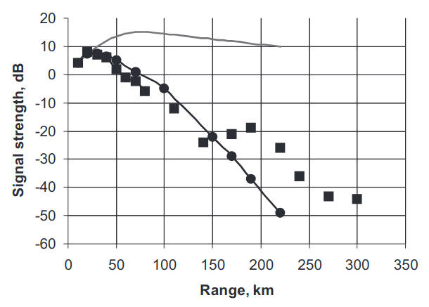
In fact, the attenuation factors, defined by both Eqs. (39) and (37), will be equal since the vertical scale of the fluctuations δε will be less than the thickness of the evaporation duct, L_z ≪ Z_s. From comparison with Eqs. (39) and (37), the value of β can be estimated as β = 0,4 which agrees well with the measurement, and, therefore, Eq. (16) can be used to estimate the attenuation of the radio wave in an evaporation duct. Figure 1 shows some results of a comparison of the field strength J in the evaporation duct relative to one in a free space at the frequency 10 GHz.

Strength of the signal — Fig. 1 Signal strength in an evaporation duct at 10 GHz: ■ Measured signal; ● Calculated, δε ≠ 0; ‒ Calculated, δε = 0

The parameter P(x, γ^′, γ):

P (x, γ^{'}, γ) = \frac{π k^{2}}{2} \int d^{2} {\vec{κ}}_{⊥} Φ_{ε} (0, {\vec{κ}}_{⊥}) \cdot \{x - {|V_{11} (κ_{z})|}^{2} \int_{0}^{x} d x^{'} e x p [j κ_{γ} (γ \frac{x^{'}}{x} + γ^{'} (1 - \frac{x^{'}}{x}))]\}, E q . 40

after integration over dγ^′ determines the attenuation exponent of the coherence function with distance x. The first term in Eq. (40) describes the attenuation of the average field due to energy transfer to the incoherent component. The second term determines the incoherent contribution of the energy scattered back to the waveguide mode in the direction of propagation.

Let us consider the intensity of the field at the point

\vec{r} = \{x, 0, z\}

produced by a point source located at

{\vec{r}}_{0} = \{0, 0, z_{0}\} .

The initial distribution of the field in Eq. (4) takes the form:

Γ_{w} (x = 0, γ^{'}, Y^{'}) = \frac{a^{2}}{4 k^{2}} ϕ_{d}^{2} (z_{0}) δ (γ^{'}) δ (Y^{'}) . E q . 41

μ_{1} = a |v| / 2, H_{s} = k Z_{s} / m, h = k ζ / m, h_{0} = k z_{0} / m, and τ_{1} = - μ_{1}^{2} 2, 338 + μ_{1}^{3} H_{s}

we obtain a solution for the intensity of the field, normalised on the intensity in a free space:

J = \frac{x^{2}}{a^{2}} {|W (x, \vec{r})|}^{2} = \frac{x^{2}}{a^{2}} Γ_{w} (x, 0, z) = \frac{k x}{8 π m^{2} τ_{1}} v^{2} (\frac{τ}{μ_{1}^{2}} - μ_{1} (H_{s} - h_{0})) \cdot v^{2} (\frac{τ}{μ_{1}^{2}} - μ_{1} (H_{s} - h)) e x p (- γ_{d} x) . E q . 42

Here, the function ϕ_d is expressed via the Airy function ν(x) of the real argument since the pole E₁ is regarded as a real one, Im{E₁} = 0. The attenuation exponent in Eq. (42) is given by:

γ_{d} = \frac{π k^{2}}{2} \int d^{2} {\vec{κ}}_{⊥} Φ_{ε} (0, {\vec{κ}}_{⊥}) [1 - |V_{11} (κ_{z})|] E q . 43

where:

{\vec{κ}}_{⊥} = \{κ_{γ}, κ_{z}\} .

γ_{d} = 0, 17 k^{2} C_{ε ⊥}^{2} {(\frac{Z_{0}}{α})}^{5 / 3} A E q . 44

where A is a constant of the order of unity, the exact value of which is defined by a true behavior of the height function ud ϕ_d(z):

A = \int_{0}^{\infty} d q \cdot q^{- 8 / 3} {[1 - |\int_{0}^{\infty} d t \cdot e^{j q t} ϕ_{d}^{2} (t)|]}^{2} . E q . 45

In the case of the bilinear model of ε_m(z), Eq. (45) takes the form:

A = \int_{0}^{\infty} d q \cdot q^{- 8 / 3} {[1 - \frac{1}{τ_{1}^{2}} |\int_{0}^{\infty} d t \cdot e^{j q t} ν^{2} (t - τ_{1})|]}^{2}, E q . 46

and calculation of Eq. (44) results in the value A = 1,51. Hence, for γ_d we obtain finally:

γ_{d} = 0, 264 k^{8 / 9} C_{ε ⊥}^{2} α^{- 5 / 3} {|v|}^{- 5 / 9} . E q . 47

Equation (47) is valid for locally uniform turbulent fluctuation δε, even when the external scales of the turbulence are infinite:

L_{z}, L_{⊥} \to \infty, σ_{ε}^{2} \to \infty .

σ_{ε}^{2}

and external scales, can be used instead of Atmospheric Boundary Layer and Basics of the Propagation Mechanismsequation. The match between models is achieved when

σ_{ε}^{2} = 1, 9 C_{ε ⊥}^{2} L_{⊥}^{2 / 3} .

The calculation of Eq. (43) can be simplified when L_z ≪ Z_s. In this case, the second term can be neglected and the attenuation factor is entirely determined by the attenuation of the coherent component of the wave field:

γ_{d} \approx γ_{s} = \frac{π κ^{2}}{2} \int d^{2} {\vec{κ}}_{⊥} Φ_{ε} (0, \vec{κ}) = 0, 374 σ_{ε}^{2} k^{2} L_{⊥} . E q . 48

α = \frac{β z_{m}}{L_{x}} = \frac{1, 32 β}{k^{2 / 3}} {|ν|}^{1 / 3} L_{x} E q . 49

and, instead of Eq. (47), we obtain:

γ_{d} = 0, 166 k^{2} C_{ε ⊥}^{2} L_{x}^{5 / 3} β^{- 5 / 3} . E q . 50

In fact, the attenuation factors, defined by both Eqs. (50) and (48), will be equal since the vertical scale of the fluctuations δε will be less than the thickness of the evaporation duct, L_z ≪ Z_s. From comparison with Eqs. (50) and (48), the value of β can be estimated as β = 0,4 which agrees well with the measurement, and, therefore, Eq. (16) can be used to estimate the attenuation of the radio wave in an evaporation duct. Figure 1 shows some results of a comparison of the field strength J in the evaporation duct relative to one in a free space at the frequency 10 GHz.

As observed from Figure 1, the calculation of the field strength in an evaporation duct using only the mean M-profile, when δε = 0, provides unrealistically high levels of the signal beyond the horizon. The curve marked by the squares is calculated with Eq. (7) using Eq. (13). The measurements of the fluctuation δε performed at the time of the radio measurements provided the following values:

C_N = 0,09 N-units cm^-1/3, L_⟂ = 48 m at a distance less than 100 km;
C_N = 0,11 N-units cm-1/3, L_⟂ = 52 m at a distance in the range between 100 and 200 km.

Here C_N = 1/2 10⁶Cε.

Figure 2 shows results of a comparison between the measured γ_m and the calculated (according to the theory provided in this section) attenuation factors γ_d at the frequency 10 GHz in the presence of an evaporation duct over the ocean.

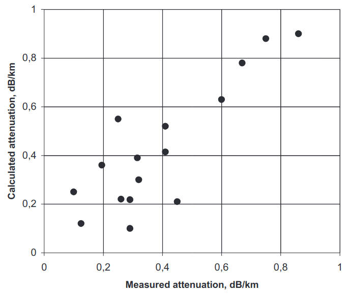
Attenuation factor — Fig. 2 Measured attenuation factor vs. that calculated according to Eq. (48)

The data were collected from 16 tests when radio measurements were performed synchronously with refractometer measurements of the fluctuations in the near-surface layer of the troposphere. The correlation coefficient between the measured and calculated values of the attenuation factor is 0,8, which suggests that the wave scattering at the fluctuations of δε provides a significant contribution to the mechanism of the radio wave propagation in an evaporation duct.

Author

Olga Nesvetailova

Freelancer

Literature

Jensen, N.O., Lenshow, D.H. An observational investigation on penetrative convection. J.Atmos.Sci., 1978, 35(10), 1924–1933.;
Monin, A.S., Yaglom, A.M. Statistical Fluid Mechanics, Vol.1, MIT Press, Cambridge, MA, 1971, p. 769.;
Gossard, E.E. Clear weather meteorological effects on propagations at frequencies above 1 GHz, Radio Sci., 1981,16(5), 589–608.;
Tatarskii, V.I. The Effects of Turbulent Atmo- sphere on Wave Propagation, IPST, Jerusalem, 1971.;
Gavrilov, A.S., Ponomareva, S.M. Turbulence Structure in the Ground Level Layer of the Atmosphere. Collected Data, Meteorology Series, No.1, Research Institute for Meteorological Information, Obninsk (in Russian), 1984.;
Kukushkin, A.V., Freilikher, V.D. and Fuks, I.M. Over-the-horizon propagation of UHF radio waves above the sea , Radiophys. Quantum Electron. (translated from Russian), Consultant Bureau, New York , RPQEAC 30 (7), 1987, 597–620.;

Footnotes