Deterministic Theory and Results of Elevated Duct Propagation

Discover a detailed comparison of experimental results with the deterministic theory of elevated duct propagation. This article examines how scattering caused by fluctuations in the refractive index excites the elevated duct, offering insightful perspectives on the validation of theoretical models through carefully conducted experiments.

СодержаниеСвернуть

Comparison of Experiment with the Deterministic Theory of the Elevated Duct Propagation
Excitation of the Elevated Duct due to Scattering on the Fluctuations in the Refractive Index

Among numerous experiments where the measured data have been compared with theoretical calculation of the propagation in the evaporation duct. We studied the height structure of the received signal strength inside the elevated duct and good agreement between theory and measured data was observed for the location of the receiving antenna inside the duct. However, in the vicinity of the channel borders the measured data exceed the levels predicted from deterministic theory.

Comparison of Experiment with the Deterministic Theory of the Elevated Duct Propagation

The measured data for frequencies 65, 170, 520 and 3 300 MHz have been compared with the theory for the respective frequencies. The elevated M-inversion forms the single mode waveguide at the frequency 65 MHz. The characteristic values of the M-profile are as follows:

Z_i = 180 m;
Z_k = 302 m;
ΔM_i = 40 M-units;

the waveguide channel is created in the interval of heights 0 < z < Zk, i. e., the duct belongs to the class of surface-based elevated ducts. Figure 1 shows very good agreement of the height dependence of the received signal strength with the theoretical calculations. It might be noted that in this frequency band the effects of scattering on the fluctuations of the refractivity are relatively small.

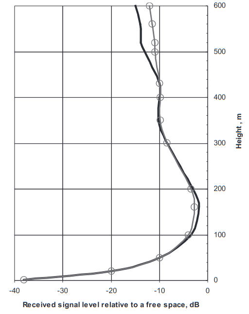
Fig. 1 Height dependence of the received field level at a distance 111,2 km from the transmitter at a frequency of 65 MHz: solid line, measured data; ○, calculated using a split-step Fourier method

Figure 2 shows the measured data for 3,3 GHz in the same duct. As observed from the figure, at this frequency the elevated duct reveals the multimode structure of the received signal level. Inside the duct the measured signal strength levels exceed the level of the field due to the condition of “normal” refraction at 50–30 dB. The results of theoretical calculation (solid line) depicted in Figure 2 show good agreement with the measured data, fitting very well between the maximum and minimum signal levels observed in the experiment inside the duct.

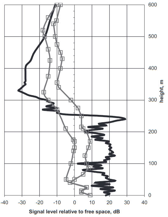
As seen from the same figure, the discrepancy between measured and predicted results becomes significant when the receiving antenna are located close to boundaries inside the duct or outside the duct. The rapid decay of the calculated signal level at heights z > 250 m is caused by a destructive interference of many modes. At the same time the amplitude of each mode may decay at a lesser rate compared with the composite of all modes. The phase relationship between modes may be distorted by non-uniformity of the refractivity structure in a horizontal plane.

The predicted path loss at frequency 3 GHz shows good agreement with the measured data for the transmitter and receiver located within the duct. Such good agreement with theory based on a rather crude model of stratified refractivity is likely due to the fact that slow variations in the refractive structure of the evaporation duct may result in “adiabatic” restructuring of the trapped modes and mutual transfer of energy between the resulting mode structure still largely formed by trapped modes. The result of this superposition in the received field strength would be close to one in the case of a horizontally uniform duct for the transmitter and receiver located far enough from the duct borders.

Figure 3 shows the results of another experiment with an elevated duct detached from the ground surface. The parameters of the M-profile in this experiment were as follows:

Z_k = 800 m;
z_min = 600 m;
ΔM_i = 20 M-units.

The transmitting antenna was located at a height 20,7 m while receiving antenna was at a height 914 m above the sea surface, i. e. outside the elevated duct.

With such placement of the receiving and transmitting antennas the trapped modes of the elevated duct cannot practically be generated by the radiating field of the transmitting antenna in such a configuration of the antennas in relation to the duct boundaries Z_k, z_min Figure 3 shows the result of the theoretical calculation of the received signal strength at frequency 3 GHz versus distance for a given placement of the antennas. As observed the calculated signal is most likely composed of the high order “leaked” modes with a rather great attenuation rate along the distance. At the same time, the measured signal level significantly exceeded that theoretically predicted from the deterministic theory of the stratified refractivity. The measured data also shown in Figure 3 do not attenuate with distance, behavior that is rather associated with trapped modes of the elevated duct.

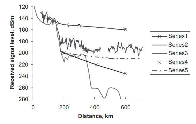
Data for M-inversion — Fig. 3 The received field strength vs. distance for elevated M-inversion at frequency 3,0877 MHz:
(1) signal strength in a free-space; (2) measured data; (3) theoretical results using averaged deterministic M-profile; (4) the level of the troposcattered signal; (5) results of the calculation using formula (50)

In order to evaluate another mechanism for long range radio wave propagation, the authors plotted in Figure 3 the level of the single-scattered field in accordance with the standard assumptions of the Booker–Gordon theory.

In a following study the authors attempted to explain the observed signal levels in Figure 3 in the above experiment by the presence of an evaporation duct at the time of mthe easurements. Nonetheless, during the radio experiment there was no adequate measurement of the meteorological data which are required to restore the M-profile near the sea surface. The authors used instead some routine meteorological data available for that area and restored three possible M-profiles of the evaporation duct, one of which provides satisfactory agreement with the measured data in Figure 3.

It might be worthwhile to consider an alternative interpretation of the measured data in the above experiment, related to excitation of the trapped modes in the elevated duct due to scattering on the turbulent fluctuations of the refractive index inside the elevated duct. The respective theory and estimates are the subject of the next section.

Excitation of the Elevated Duct due to Scattering on the Fluctuations in the Refractive Index

Consider the piece-wise linear mode of the M-profile, introduced at the beginning of this chapter, Figure 1, and assume Z_s = 0, ΔM = 0. In this section we investigate the mechanism of excitation of the elevated duct that can be formulated as follows:

The characteristic values of the thickness, Z_k – Z_i, of the elevated M-inversion and depth, ΔM_i, in most cases are themselves sufficient to ensure a waveguide mechanism for radio wave propogation in the range of 1–10 GHz of the frequency spectrum.

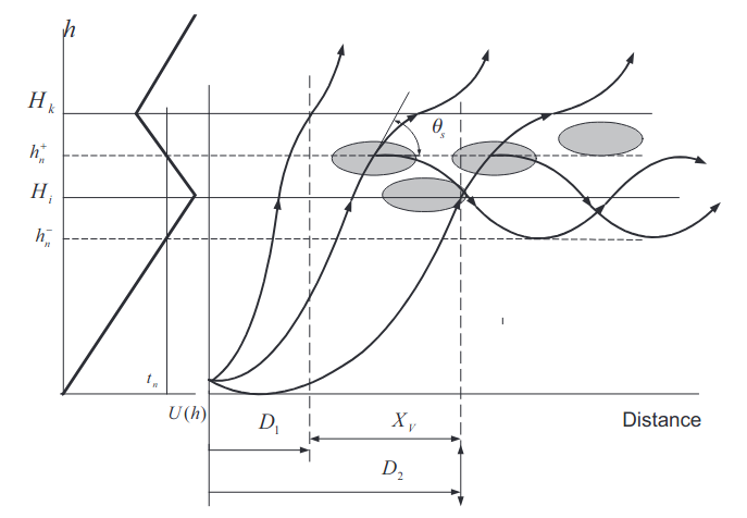
As discussed in Atmospheric Boundary Layer and Basics of the Propagation Mechanisms“Atmospheric Boundary Layer and Key Propagation Mechanisms”, the elevated duct location is defined in the interval of heights Z_min ≤ z ≤ Z_k. The efficiency of the excitation of the guided waves nonetheless depends on the position of the transmitting antenna relative to the duct boundaries. If the antenna hight z₀ is outside the duct, say z₀ < Z_min, it is “impossible”, from the geometric optic point of view, to excite the guided waves. This means that the radiated field of the direct wave propagates through the elevated refractive layer experiencing slight refraction within, Figure 4. In this case the trapping of the waves inside the elevated duct is only possible due to scattering on the fluctuations of the refractive index, Figure 4.

The distances of interest are far beyond the horizon relative to the scattering volume, therefore we take into account only a single scattering into trapped modes of the elevated duct. For the same reason, the size of the scattering volume in the heights is limited by the interval of localisation of the trapped mode, i. e., Z_min ≤ z ≤ Z_k. Let us assume that the width of the antenna pattern ha in azimuth is wide enough, i. e:

ϑ_{a} D ≫ L_{| |} E q . 1

where D is the distance between the transmitter and the scattering volume, L_|| is an external scale of the fluctuations in de in the plane (x, γ). In the current estimate of the scattering field we use an approximation for a free-space attenuation function W₀ of the direct wave. In this approximation for W₀ we do not take into account refraction (other than normal refraction) along the path between the transmitting antenna and a point within the scattering volume. In the problem of interest the impact of refraction is insignificant, since there is no trapping of the incident direct wave within the elevated refractive layer. We also will not take into account the effect of the boundary z = 0 on the scattered field. The presence of the interface z = 0 leads to a lobed structure of the incident field. Such a complication, while easy to account for, is not worthwhile in the evaluation of the effect on the order of magnitude, which is the purpose of this investigation. Therefore, we take the artificial case of a grounded antenna z = for further study in this section.

Excitation of elevated duct — Fig. 4 Schematic diagram of excitation of the elevated duct via a scattering mechanism

The Green function of the scattered field we define as the superposition (Impact of Elevated M-inversions on the UHF/EHF Field Propagation beyond the Horizon“in this equation”) of the trapped modes of the elevated duct. The height-gain functions χ_n(s) are then defined by Impact of Elevated M-inversions on the UHF/EHF Field Propagation beyond the Horizon“this equation” within the scattering volume.

Another important assumption is that the major contribution to scattering comes from the inhomogeneities of δε in the vicinity of the upper boundary of the elevated refractive layer, i. e., with Z_i ≤ z ≤ Z_k. This assumption is founded on observations of the sharp increase in intensity of the fluctuation of δε in the vicinity of the upper boundary of the elevated layer, which is also associated with the upper boundary of the marine boundary layer. As a result, scattering into the trapped mode with number n is chiefly produced by the inhomogeneities located in the vicinity of the upper turning point

z_{n}^{+}

of the wave associated with the nth mode, Figure 4:

z_{n}^{+} = \frac{m}{k μ_{3}^{3}} (U_{i} - t_{n} - μ_{3}^{3} H_{i}) . E q . 2

In fact, the upper limit of integration η⁺ over the height of the scattering volume for the nth mode is effectively limited by the height of the turning point

z_{n}^{+}

and, from below, by the characteristic scale Λ_z of the oscillations in the height-gain function Λz ~ m/kμ₃. Let us demand the following inequalities to be true:

L_{z} ≪ a / m t_{n} = Λ_{x}, L_{| |} ≪ X_{V} = D_{2} - D_{1} E q . 3

where L_z is the characteristic external scale of the fluctuations in δε. The parameter Λ_x in Eq. (6) is a characteristic scale of diffraction of the mode field due to the curvature of the earth, in the 10 GHz range Λx ~ 10 km; X_V is the length of the scattering volume, Figure 4, normally about several tens of km. Under condition:

θ_{r} ≪ θ_{s} E q . 4

where θ_s = λ/L_z is the scattering angle in the vertical plane and

θ_{r} = \sqrt{Z_{i} / 2 a}

is the characteristic angle of refraction. The wave front of the incident wave has to be turned to an angle θ_r in order for that wave to be trapped in the elevated duct. The inequality (4) means that the angular width of the scattering exceeds the characteristic angle of refraction. In this case, the inequality:

\frac{Λ_{z}}{2 Z_{i}} \frac{θ_{r}^{2}}{θ_{s}^{2}} ≪ 1 E q . 5

holds and we can neglect the changes in the characteristic angle of refraction θ_r within the scattering volume. Let us estimate the common values involved in problem formulation: the height of the elevated layer Z_i is normally about Z_i ~ 102 – 103 m; the Fresnel zone size:

\sqrt{λ D} ≅ λ^{1 / 2} {(2 a Z_{i})}^{1 / 2}

is about 100 m in the 10 GHz range; the external size L_|| of the inhomogeneities δε in the horizontal plane is about L_|| ≈ 5·10²-10³ m at heights of the order of Z_i; the vertical scale L_z is much smaller and is of the order of tens of meters because of the strong anisotropy present in vicinity the of the upper border of the atmospheric boundary layer. We can also assume that:

Λ_{z} ≫ L_{z} E q . 6

which is most certainly satisfied for lower-order trapped modes, and then the intensity of the single-scattered field can be obtained in the form:

J = <{|W|}^{2}> = 0, 07 k^{- 2 / 3} C_{ε}^{2} α^{- 5 / 3} {(2 m)}^{11 / 3} (\frac{g_{23}}{ξ_{v}}) \cdot \sum_{n = 1}^{N} χ_{n} (z) e^{- γ_{n} ξ_{v}} (ξ_{2, n}^{2} - ξ_{1, n}^{2}) {(\frac{h_{n}^{+}}{ξ_{n}^{+}})}^{- 8 / 3} . E q . 7

Here:

h_{n}^{+} = k z_{n}^{+} / m, ξ_{n}^{+} = (ξ_{1, n} + ξ_{2, n}) / 2, g_{23} = {(μ_{2} μ_{3})}^{6} / {(μ_{2}^{3} + μ_{3}^{3})}^{2}, C_{ε}

is a structure constant of the fluctuations of δε in the vicinity of the upper border of the marine boundary layer z ~ Z_i. The parameters ξ_1,n, ξ_2,n determine the non-dimensional borders of the effective scattering volume. To define them we use the geometry of the problem. Let us assume that the half-width of the antenna pattern in the vertical plane (E-plane) (x, z) is equal to θ_e.

The ray which departs from the source at an angle θ_e can be related to the stationary value of the non-dimensional energy t = m² E/k² (see Understanding Parabolic Approximation in Wave Propagation: Analytical Methods and Applications“Parabolic Approximation to a Wave Equation in a Stratified Troposphere Filled with Turbulent Fluctuations of the Refractive Index”), equal to

t_{1} = - m^{2} θ_{e}^{2}

(Understanding Parabolic Approximation in Wave Propagation: Analytical Methods and Applicationsanalog of the formula). For the ray tangential to the earth’s surface, as follows from Understanding Parabolic Approximation in Wave Propagation: Analytical Methods and Applications“Parabolic Approximation to a Wave Equation in a Stratified Troposphere Filled with Turbulent Fluctuations of the Refractive Index”, the stationary value is t = t₂ = 0.

The ray with stationary value t₁ reaches the upper

h_{n}^{(+)}

and lower

h_{n}^{(1)}

heights of the turning level for mode of number n and the respective distances:

ξ_{1, n}^{(-)} = \frac{1}{μ_{2}^{3}} \sqrt{t_{n} - t_{1}}, E q . 8

ξ_{1, n}^{(+)} = \frac{1}{μ_{2}^{3}} \sqrt{U_{i} - t_{1}} + \frac{1}{μ_{3}^{3}} (\sqrt{U_{i} - t_{1}} - \sqrt{t_{n} - t_{1}}), E q . 9

and the heights

h_{n}^{(+)}, h_{n}^{(-)}

are given by:

h_{n}^{(+)} = \frac{1}{μ_{3}^{3}} (U_{i} - t_{n} + μ_{3}^{3} H_{i}), E q . 9

h_{n}^{(-)} = \frac{1}{μ_{2}^{3}} t_{n} .

The near boundary ξ_1,n of the scattering volume in Eq. (7) can then be defined as:

ξ_{1, n} = (ξ_{1, n}^{(-)} + ξ_{1, n}^{(+)}) / 2 .

The far boundary ξ_2,n can be defined in similar way using the Eq. (8) with t₁ replaced by t₂ = 0.

Curve (5) in Figure 3 shows the estimate of the scattered field in the elevated duct using Eq. (7) with the value of structure constant:

C_{ε}^{2} = 10^{- 15} c m^{- 2 / 3} .

As observed from the figure, the strength of the estimated scattered field is 25 dB less than the level of the measured signal. This might be explained by underestimation of the intensity of the fluctuations in refractive index in the vicinity of tZ_k, which potentially can reach a value of two orders of magnitude higher than the value:

C_{ε}^{2} = 10^{- 15} c m^{- 2 / 3} .

Such values of

C_{ε}^{2}

have been reported in Refs. Of course, any attempt to match the theory (7) with the measured data would be speculative, since information about fluctuations in the refractive index was not reported in Refs. The main purpose of the above comparison is to give a somewhat different explanation of the mechanism of the propagation that can hardly be explained by the deterministic model of a stratified troposphere.

Author

Olga Nesvetailova

Freelancer

Literature

Wait, J.R. Electromagnetic Waves in Stratified Media, Oxford, Pergamon Press, Oxford, 1962, 372 pp.;
Bremmer, H. Terrestrial Radio Waves, Elsevier, New York, 1949, 343 pp.;
Dresp, M.R., Rather A.S. Tropospheric duct propagation beyond the horizon, Proc. URSI Commission, Sect. F. Open Symp., La Baule, France, 1977, Pt.1, pp. 31–36.;
Baz, A.I., Zeldovich, Y.B., Perelomov, A.M. Scattering, Reactions and Decays in. Nonrelativistic Quantum Mechanics, Academic Press, New York, 1980.;
Ott, R.H. Roots of the modal equation for em wave propagation in a tropospheric duct, J. Math. Phys., 1980, 21 (5), 1256–1266.;
Migliora, C.G. Felsen, L.B., Cho, S.H. High Frequency propagation in elevated tropospheric duct, IEEE Trans. Antennas Propagation, 1982, 30, 1107–1120.;
Baumgartner, Jr., G.B., Hitney, H.V., Pappert R.A. Duct propagation modelling for the integrated refractive effects prediction system (IREPS)., Proc. IEE, 1983,130, Pt.F, 630–642.;
Felsen, L.B. Hybrid ray-mode fields in inhomogeneous waveguides and ducts, J. Acoust. Soc. Am., 1981, 69 (2), 352–361.;
Marcus, S.V. A model to calculate em fields in tropospheric duct environments at the frequencies through SHF, Radio Sci., 1982, 17, 895–901.;
Pappert, R.A., Goodhart, C.L. Case study of beyond-the-horizon propagation in tropospheric duct environments, Radio Sci., 1977, 12 (1), 75–81.;
Kukushkin, A.V., Sinitsin, V.G. Rays and modes in non-uniform troposphere, Radio Sci., 1983, 18 (4), 573–581.;
Guinard, N.W., Ransone, J., Randall, D. et al. Propagation through an elevated duct. Tradewind 3, IEEE Trans. Antennas Propagation, 1964, 12 (4), 479–453.;
Hitney, H.V., Pappert, R.A., Hattan, C.P. Evaporation duct influences on beyond-the-horizon high altitude signals, Radio Sci., 1978, 13 (4), 669–675.;
Chang, H.T. The effect of tropospheric layer structures on long-range VHF radio propagation, IEEE Trans. Antennas Propagation, 1971, 19 (6), 751–756.;
Booker, H., Gordon, W. A theory of radio scattering in the troposphere, 1950, Proc. IRE, 1950, 38 (4), 401–412.;
Gavrilov, A.S., Ponomareva, S.M. Turbulence Structure in the Ground Level Layer of the Atmosphere, Collected Data, Meteorology Series, 1984, No.1, Research Institute for Meteorological Information, Obninsk, (in Russian).;
Deardorff, J.W, Willis, G.E. Further results from a laboratory model of the convective boundary layer, Bound. Layer Met., 1985, 35, 205–236.;

Footnotes