Elevated M-Inversions and EHF/UHF Field Propagation

Explore the impact of elevated M-inversions on UHF/EHF field propagation beyond the horizon, examining atmospheric effects and anomalous radio frequency behavior.

The elevated refractive layer, the so-called M-inversion, is frequently associated with an anomalousy high level of the received signal at UHF frequencies over the horizon. It is apparent that the methods of prediction of either the parameters of the elevated layer or the signal level are needed in many applications, such as radar, surveillance and communications.

The methods of the analytical solutions to the problem of wave propagation in the presence of elevated M-inversion are less well developed than those applied to propagation in an evaporation duct. The major reason for this is that such a waveguide has a multi-mode or multi-ray nature that, in turn, may require a different approach to obtaining the analytical solution, depending on the geometry of the problem (positions of the transmitter and receiver relative to the elevated duct “boundaries”, range and frequency).

For instance, when the transmitter and receiver are based close to the ground with the distance between them

x ≪ 2 \sqrt{2 a Z_{i}},

see Figure 1, where Z_i is the height of the minimum in the M-profile of the refractivity, the most effective approach is to apply the method of multiple reflections, that, in turn leads to the approximation of the geometrical optic with k → ∞. In contrast, at longer distances, the most effective method uses normal waves providing the modal representation of the wave field.

In a sub-tropical region of the world’s oceans both evaporated and elevated ducts may exist simultaneously thus complicating the situation. In Refs this situation is analysed by applying the normal wave method to the M-profile approximated by a piece-wise linear profile. An alternative approach is described in Hybrid Representation in Action: Fock’s Contour Integral and the Attenuation Factor“Exploring Hybrid Representation for the Attenuation Factor”, where the contribution of evaporation duct is presented by trapped modes while the reflection from elevated M-inversion is analysed in terms of geometric optics.

The modal representation of the wave field for the case of elevated M-inversion is presented in this article. Hybrid Representation in Action: Fock’s Contour Integral and the Attenuation Factor“Exploring Hybrid Representation for the Attenuation Factor” introduces the hybrid, ray and modes, representation of the wave field in the problem of a two-channel system. Some results of the measurements versus prediction are discussed in Comparison of Experimental Results with the Deterministic Theory of Elevated Duct Propagation“Deterministic Theory and Results of Elevated Duct Propagation” and, finally, in Comparison of Experimental Results with the Deterministic Theory of Elevated Duct Propagation“Deterministic Theory and Results of Elevated Duct Propagation”, we introduce a method of estimating the excitation of the elevated duct due to scattering of the direct wave on the fluctuations in refractivity in the vicinity of the upper boundary of the atmospheric boundary layer.

Modal Representation of the Wave Field for the Case of Elevated M-inversion

Consider a piece-wise linear model of the M-profile as shown in Figure 1 and introduce the dimensionless coordinates ξ = mx/a, h = kz/m.

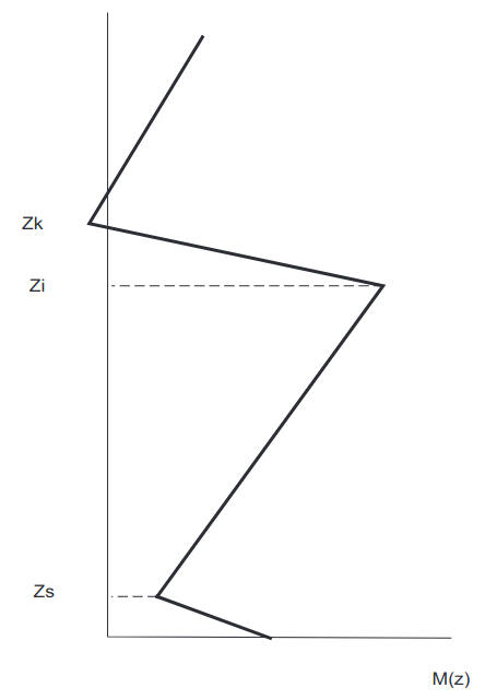
The parameters of the M-profile can be expressed in terms of h-coordinates and the scaled potential U(h) = 2m²10^-6M(z):

H_k = kZ_k/m;
H_i = kZ_i/m;
H_s = kZ_s/m;
U_k = 2m²10^-6M(Z_k);
U_i = 2m²10^-6M(Z_i);
U₀ = 2m²10^-6ΔM.

Let us also introduce the gradients of the M-profile in each of the layers between Z_s, Z_i and above Z_k respectively:

G₂ = dM/dz, with Z_s < z < Z_i;
G₄ = dM/dz, with z > Z_k.

The respective gradients of the dimensionless profile U(h) are given by:

μ_{1}^{3} = U_{0} / H_{s}, μ_{2}^{3} = a \cdot 10^{- 6} G_{2}, μ_{3}^{3} = (U_{i} - U_{k}) / (H_{k} - H_{i}), μ_{4}^{3} = a \cdot 10^{- 6} G_{4} .

Following the approach described in Understanding Parabolic Approximation in Wave Propagation: Analytical Methods and Applications“Parabolic Approximation to the Wave Propagation”, we expand the attenuation factor W(ξ, h, h₀) over the set of eigenfunctions of a continuum spectrum. Using the results of Green Function for a Parabolic Equation in a Stratified Medium“Parabolic Approximation to the Wave Propagation” and introducing the dimensionless “energy” t = m²E/k² we obtain:

W (ξ, h, h_{0}) = e^{- j \frac{π}{4}} \int_{- \infty}^{\infty} d t Ψ (t, h) Ψ^{*} (t, h_{0}) e^{j ξ t} E q . 1

where the eigenfunction Ψ(t, h) obeys the equation:

\frac{d^{2} Ψ}{d h^{2}} + [U (h) - t] Ψ = 0 E q . 2

and the boundary conditions:

Ψ (t, 0) = 0 a n d Ψ (t, \infty) = 0 . E q . 3

As known from analogy with a quantum-mechanical problem, the solution to Eq. (2) is given by a superposition of the waves, outgoing (χ⁺) to infinity (h → ∞) and incoming (χ^–) from infinity:

Ψ (t, h) = \frac{1}{2 \sqrt{π μ_{4}}} [χ^{-} (t, h) - S (t) χ^{+} (t, h)] . E q . 4

It is also observed that χ^–(t, h) = (χ⁺(t, h))^*, where the sign * indicates a complex conjugate. The factor

\frac{1}{2 \sqrt{π μ_{4}}}

in Eq. (4) comes from a delta-function normalisation of the eigenfunction of the continuum spectrum, Understanding Parabolic Approximation in Wave Propagation: Analytical Methods and Applications“Green Function for a Parabolic Equation in a Stratified Medium”. From the boundary condition (3) we have:

S (t) = \frac{χ^{-} (t, 0)}{χ^{+} (t, 0)} . E q . 5

Given the linear approximation to the M-profile in each of the layers: H_s < h ≤ H_i H_s < h ≤ H_i, H_i < h ≤ H_k and h > H_ki the solution for χ^± can be presented via superposition of the Airy–Fock function. Taking into account the continuity of both the function v and its derivative at the boundaries of the layers with constant gradient of U(h), the outgoing wave can be written as follows:

1 With h > H_k:

χ^{+} (h) = w_{1} (\frac{t - U (h)}{μ_{4}^{2}}) . E q . 6

2 with h_k ≥ h > h_i:

χ^{+} (h) = A \{w_{1} (\frac{t - U (h)}{μ_{3}^{2}}) + R_{k} w_{2} (\frac{t - U (h)}{μ_{3}^{2}})\} E q . 7

where:

A = \frac{w_{2} (x_{k}^{+})}{w_{1} (x_{k}^{-}) + R_{k} w_{2} (x_{k}^{-})}, E q . 8

R_{k} = - \frac{w_{2}^{'} (x_{k}^{-}) + Q_{k} w_{2} (x_{k}^{-})}{w_{1}^{'} (x_{k}^{-}) + Q_{k} w_{1} (x_{k}^{-})} . E q . 9

Here:

x_{k}^{+} = \frac{t - U_{k}}{μ_{4}^{2}}, x_{k}^{-} = \frac{t - U_{k}}{μ_{3}^{2}}, R_{k}

is a reflection coefficient of the wave incident to the boundary h = H_k from h < H_k, the parameter Q_k is the surface impedance at the boundary h = H_k and is given by:

Q k = \frac{μ_{4}}{μ_{3}} \frac{w_{1}^{'} (x_{k}^{+})}{w_{1}^{'} (x_{k}^{-})} . E q . 10

3 with H_i ≥ h > H_s:

χ^{+} (h) = B \{w_{1} (\frac{t - U (h)}{μ_{2}^{2}}) + R_{i} w_{2} (\frac{t - U (h)}{μ_{2}^{2}})\} E q . 11

where:

B = A \frac{w_{2} (x_{i}^{+}) + R_{k} w_{1} (x_{i}^{+})}{w_{1} (x_{i}^{-}) + R_{i} w_{2} (x_{i}^{-})}, E q . 12

R_{i} = - \frac{w_{1}^{'} (x_{i}^{-}) + Q_{i} w_{1} (x_{i}^{-})}{w_{2}^{'} (x_{i}^{-}) + Q_{k} w_{2} (x_{i}^{-})}, E q . 13

Q_{i} = \frac{μ_{3}}{μ_{2}} \frac{w_{1}^{'} (x_{i}^{+}) + R_{k} w_{1} (x_{i}^{+})}{w_{2}^{'} (x_{i}^{-}) + R_{k} w_{2} (x_{i}^{-})}, E q . 14

Here:

x_{i}^{+} = t - U_{i} / μ_{3}^{2}, x_{i}^{-} = t - U_{i} / μ_{2}^{2},

the other parameters have the same meaning as above.

4 With h ≤ H_s:

χ^{+} (h) = C \{w_{2} (\frac{t - U (h)}{μ_{1}^{2}}) + R_{s} w_{1} (\frac{t - U (h)}{μ_{1}^{2}})\} E q . 15

where:

C = B \frac{w_{1} (x_{s}^{+}) + R_{i} w_{2} (x_{s}^{+})}{w_{2} (x_{s}^{-}) + R_{s} w_{1} (x_{s}^{-})}, E q . 16

R_{s} = - \frac{w_{2}^{'} (x_{s}^{-}) + Q_{s} w_{2} (x_{s}^{-})}{w_{1}^{'} (x_{s}^{-}) + Q_{s} w_{1} (x_{s}^{-})}, E q . 17

Q_{i} = - \frac{μ_{2}}{μ_{1}} \frac{w_{1}^{'} (x_{s}^{+}) + R_{i} w_{1} (x_{s}^{+})}{w_{2}^{'} (x_{i}^{-}) + R_{k} w_{2} (x_{i}^{-})} . E q . 18

Here

x_{s}^{+} = τ / μ_{2}^{2}, x_{s}^{-} = τ / μ_{1}^{2},

, the other parameters have the same meaning as above.

The solution to W(ξ, h, h₀) is obtained in principle and given by Eqs. (1)–(18). However, the direct calculation of Eq. (1) is not practical because of the problem of convergence. Therefore, a significant amount of research has been dedicated to finding effective methods of calculating the electromagnetic field in the presence of elevated M-inversion.

Here we consider a modal representation of the attenuation function W(ξ, h, h₀) in a two-channel system when both elevated and surface-based M-inversion are present. In this approach, UHF Propagation in an Evaporation Ductthe integral is calculated as a sum of the residue at the poles of the S-matrix in the upper half-space of variable t. Taking into account Eqs. (5)–(18) we obtain the expression for the S-matrix in this particular problem:

S = - R_{g} \frac{A^{*} w_{2}^{2} (x_{s}^{-}) \cdot (1 - R_{i}^{*} T_{s}^{-}) \cdot (1 - R_{i}^{*} T_{s}^{+}) \cdot (1 - R_{i}^{*} R_{g}^{*})}{A w_{1}^{2} (x_{s}^{-}) \cdot (1 - R_{i} T_{s}^{+}) \cdot (1 - R_{i} T_{s}^{-} ＊) \cdot (1 - R_{i} R_{g})} E q . 19

where:

R_g = -w₁(x₀)/w₂(x₀) is the reflection coefficient of the ground;
$x_{0} = t - U_{0} / μ_{1}^{2}, T_{s}^{+} = - w_{2} (x_{s}^{+}) / w_{1} (x_{s}^{-})$
is the reflection coefficient of the wave incoming from the upper space from the boundary h = H_s with ideal boundary conditions on it;
$T_{s}^{-} = - w_{1} (x_{s}^{-}) / w_{2} (x_{s}^{+})$
is a similar coefficient of reflection from the boundary h = H_s,but for the wave incoming from the space below the boundary h = H_s.

The resonant terms in the denominator of the S-matrix determine the spectrum of the normal waves in a two-channel system. Apparently, the propagation constants of the normal waves are defined by the position of the poles of the S-matrix in the t-plane. The waves trapped in an evaporation duct (surface-based M-inversion) have propagation constants tn in the interval Re t_n ∈ (0, U₀). Waves localised in the elevated duct between H_s and H_k have propagation constants t_n in the interval Re t_n ∈ (0, U_i). And, finally, the normal waves localised in a channel formed by the ground surface h = 0 and the upper boundary of the elevated layer h = H_k are in the interval Re t_n ∈ (U_k, 0).

Now we consider the resonant terms of the S-matrix in more detail and assume that Uk > 0. The resonant term

1 - R_{i} T_{s}^{+}

determines the spectrum of the normal waves for the elevated channel with boundaries h = H_s and h = H_k. With U₀ ≠ 0 localisation of the modes in the surface-based channel is possible, in principle, and the spectrum of these modes is defined by the equation 1 – R_sR_g = 0. In the case where U_kU₀, both series of propagation constants are clearly separated in the wave-number space. More detailed analysis of this case is provided in Hybrid Representation in Action: Fock’s Contour Integral and the Attenuation Factor“Exploring Hybrid Representation for the Attenuation Factor”. Now we concentrate on the modes of the elevated channel (duct). The characteristic equation for the spectrum of propagation constants is given by:

1 - R_{i} T_{s}^{+} = 0 . E q . 20

With

τ / μ_{2}^{2} ≫ 1

we can estimate:

T_{s}^{+} = - 1 + O (e^{- \frac{4}{3} t_{n}^{3 / 2} / μ_{2}^{2}})

and Eq. (20) can then be reduced to 1+R_i = 0. Assume that the propagation constants of interests are such that:

R e t_{n} - U_{k} / μ_{2}^{2} ≫ 1 .

These normal waves experience complete reflection from the boundary h = Hk, in fact the respective rays turn back long before reaching the boundary H_k. The reflection coefficient can then be estimated as R_k ≈ -1. Taking into account Eq. (12) for R_i we can obtain instead of Eq. (20) the following characteristic equation for the waves trapped in an elevated duct:

v^{'} (x_{i}^{-}) + q_{i} v (x_{i}^{-}) = 0 E q . 21

where:

q_{i} ≅ μ_{3} / μ_{2} v^{'} (x_{i}^{+}) / v (x_{i}^{+}), v (x) = (1 / 2) j [w_{1} (x) - w_{2} (x)] .

Equation (21) can be further simplified using the asymptotic formulas for the Airy function v. The result is given by:

\sin (ς_{i}^{+} + ς_{i}^{-} + \frac{π}{2}) = 0, E q . 22

where:

ς_{i}^{+} = \frac{2}{3 μ_{3}^{3}} {(U_{i} - t)}^{3 / 2}, ς_{i}^{-} = \frac{2}{3} μ_{2}^{3} {(U_{i} - t)}^{3 / 2} .

The solution to Eq. (22) provides a spectrum of the propagation constants t_n of the elevated duct:

t_{n} = U_{i} - {[\frac{3}{2} \frac{{(μ_{2} μ_{3})}^{3}}{μ_{2}^{3} + μ_{3}^{3}} π (n - \frac{1}{2})]}^{2 / 3} . E q . 23

As observed, Eq. (23) is obtained by neglecting the leaking of the modes into the space outside the duct. The number N₁ of trapped modes is limited by the condition t_n > U_k, therefore:

N_{1} = entier [\frac{2}{3} \frac{μ_{2}^{3} + μ_{3}^{3}}{(μ_{2} μ_{3})} {(U_{i} - U_{k})}^{3 / 2} + \frac{1}{2}] . E q . 24

Counting the next terms of the asymptotic for both

T_{s}^{+}

and R_k we can obtain from Eq. (20) some correction terms to the propagation constants t_n (23). These correction terms provide an estimate for a phase shift and attenuation factor for the modes due to the limited thickness of the potential barrier. Omitting the simple but cumbersome calculations we provide the final result for the imaginary part of the propagation constants:

γ_{n} = Im t_{n} = \frac{1}{4} \frac{μ_{2}^{3} + μ_{3}^{3}}{{(μ_{2} μ_{3})}^{3}} \exp \{- \frac{4}{3} \frac{μ_{3}^{3} + μ_{4}^{3}}{{(μ_{3} μ_{4})}^{3}} {(t_{n} - U_{k})}^{3 / 2}\} . E q . 25

Let us consider another situation and assume now that U_k < 0. We pay attention to the modes of the channels formed by the earth’s surface h = 0 and the upper boundary of the M-inversion, h = H_k. As discussed above, the propagation constants of these modes lie in the interval Re t_n ∈ (U_k, 0). The spectrum of the propagation constant is determined by the characteristic equation 1 – R_sR_g = 0. Using asymptotic expressions for Airy functions we obtain:

R_{s} ≅ R_{i} D e^{- j δ}, E q . 26

R_{g} ≅ - \exp [j \frac{π}{2} + j \frac{4}{3 μ_{1}^{3}} {(U_{0} - t)}^{3 / 2}]

where:

δ = π + \frac{4}{3} \frac{μ_{2}^{3} + μ_{3}^{3}}{μ_{2}^{3} μ_{3}^{3}} (- t), D = \frac{1}{2 - R_{i} T_{s}^{+}},

T_{s}^{+} ≅ - \exp [j \frac{π}{2} - j \frac{4}{3 μ_{2}^{3}} {(- t)}^{3 / 2}] .

Let us expand the term D into a series:

D = \sum_{m = 0}^{\infty} {(- 1)}^{m} {(1 - R_{i} T_{s}^{+})}^{m} . E q . 27

The series (27) takes into account the multiple effect of secondary reflection of the waves in the channel H_s ≤ h ≤ H_k due to a leakage of the energy of the normal waves localised in the channel 0 < h ≤ H_k due to partial reflection from the boundary h = Hs. In the first and rough approximation this effect of mutual coupling of two channels can be neglected, at least this approximation will be good enough for |Re t_n| ≫ 1. Under this condition we can retain only the first term in series (27). As a result we obtain:

1 - R_{s} R_{g} \approx 1 - R_{i} R_{g} e^{- j δ} = 0 . E q . 28

The last equation can be further simplified to the form:

\frac{2}{3} \frac{μ_{2}^{3} + μ_{3}^{3}}{μ_{2}^{3} μ_{3}^{3}} {(U_{i} - t_{n})}^{3 / 2} + \frac{2}{3 μ_{1}^{3}} {(U_{0} - t_{n})}^{3 / 2} - \frac{2}{3} \frac{μ_{2}^{3} + μ_{1}^{3}}{μ_{2}^{3} μ_{1}^{3}} {(- t_{n})}^{3 / 2} = π (n - \frac{1}{4}) . E q . 29

The limiting case when surface M-inversion is absent is accounted for by Eq. (29) if we assume that U₀ = 0. We can also observe that the number n satisfying Eq. (29) starts from n = N₁ + N₂ + 1, where N₂ is the number of modes trapped in a surface-based channel, 0 < h ≤ H_s.

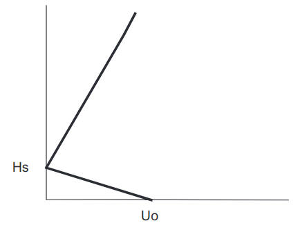
To conclude, we may state that the characteristic equations (20) and (29) determine the limited, yet large, (for high frequencies and strong inversions of temperature) set of trapped modes in a two-channel system. While in the general case the two modal series in the evaporation and the elevated duct are coupled, for modes localised deep in respective channels the mutual coupling can be neglected in the first approximation. In this way, the trapped modes of the evaporation duct can be estimated as the modes formed by a surface-based inversion only, Fig. 2, and the analysis is similar to that provided in UHF Propagation in an Evaporation Duct“Exploring UHF Propagation in Evaporation Ducts”.

Surface-based inversion — Fig. 2 Isolated surface-based M-inversion

Let us obtain a residue of the integrand in Eq. (1) in the pole of the S-matrix. Utilising the asymptotic expression for Airy functions incorporated into Ψ(t, h) and Ψ^*(t, h₀), the residue with Re t_n > U_k is truncated to:

R e s Ψ (t, h) Ψ^{*} {(t, h_{0})}_{t = t_{n}} = 2 j Im \{t_{n}\} χ^{+} (t_{n}, h) χ^{+} (t_{n}, h_{0}) E q . 30

Next we obtain an asymptotic expression for the height-gain functions χ⁺(t_n, h). First, define the coefficients (8) and (12) for Re t_n > U_k:

A (t_{n}) \approx j \sqrt{\frac{μ_{4}}{μ_{3}}} \exp (\frac{∆}{2}) E q . 31

where:

∆ = \frac{4}{3} \frac{μ_{3}^{3} + μ_{4}^{3}}{μ_{3}^{3} μ_{4}^{3}} {(t_{n} - U_{k})}^{3 / 2}

and, for Re t_n > 0:

B (t_{n}) \approx A \sqrt{\frac{μ_{3}}{μ_{2}}} \frac{1}{\cos (n π)} E q . 32

For 0 > Re t_n > U_k:

B (t_{n}) \approx 2 j \sqrt{\frac{μ_{3}}{μ_{2}}} \sin (\frac{3}{2 μ_{2}^{3}} {(U_{i} - t_{n})}^{3 / 2} + \frac{π}{4}) [1 - \exp \{j \frac{4}{3 μ_{2}^{3}} {(U_{i} - t_{n})}^{3 / 2} + j \frac{π}{2}\}] \cdot \exp \{- j \frac{2}{3 μ_{2}^{3}} {(U_{i} - t_{n})}^{3 / 2} - j \frac{π}{4}\} . E q . 33

While obtaining Eq. (32) we take into consideration that R_i(t_n) = -1 at the pole. Assume that there is no evaporation duct present, i. e. H_s = 0, U₀ = 0, and consider a height-gain function χ^–(t_n, h) with h → 0 for 0 > Re t_n > U_k. As follows from Eq. (11):

χ^{+} (t_{n}, h = 0) = 2 B \cos (S_{1} - δ) \exp (j δ) E q . 34

where:

S_{1} = \frac{2}{3 μ_{2}^{3}} {(- t_{n})}^{3 / 2} + \frac{π}{4}, δ = \frac{2}{3} \frac{μ_{2}^{3} + μ_{3}^{3}}{μ_{2}^{3} μ_{3}^{3}} {(U_{i} - t_{n})}^{3 / 2} .

Taking into account that at the pole, as follows from Eq. (22) with U₀ = 0, the arguments of the cosine in the term S₁ – δ = -nπ + π/2, we obtain the boundary condition of interest, χ⁺(h = 0) = 0. With U₀ ≠ 0 and Re t_n < 0, from Eq. (15) it follows that:

χ^{+} (t_{n}, 0) \approx \cos [\frac{2}{3 μ_{1}^{3}} {(U_{0} - t_{n})}^{3 / 2} - \frac{2}{3} \frac{μ_{1}^{3} + μ_{2}^{3}}{μ_{1}^{3} μ_{2}^{3}} {(- t_{n})}^{3 / 2} - \frac{π}{4}] . E q . 35

The equation for the poles takes the form R_sR_g = 1 in this case. The relationship between R_s and R_g is given by Eq. (26) from which we obtain that the argument of the cosine in Eq. (35) has the value nπ + π/2 at the pole and, therefore χ⁺(t_n, 0) = 0.

In the case of positive Re t_n > 0, |t_n| ≫ 1, the behavior of the height-gain function χ⁺(t_n, h) with h → 0 is governed by the exponent factor:

χ^{+} {(t_{n}, h)}_{h \to 0} \approx e x p (- \frac{2}{3 μ_{2}^{3}} {(- t_{n})}^{3 / 2}) \to 0

and the boundary condition at h = 0 is satisfied asymptotically.

Finally, we can present an explicit expression for the attenuation function W(ξ, h, h₀) over the sum of the normal waves that can be used for computer calculation:

W (ξ, h, h_{0}) = e^{j π / 4} \sqrt{\frac{ξ}{π}} \frac{1}{4 μ_{4}} \frac{μ_{2}^{3} μ_{3}^{3}}{μ_{2}^{3} + μ_{3}^{3}} \sum_{n = 1}^{N} e^{j ξ t_{n} - γ_{n} ξ} χ_{n} (h) χ_{n} (h_{0}) . E q . 36

The number of trapped modes N is determined by the number of real roots of Eqs. (22) and (29). The eigenfunction χ_n(h) is given by the following equations:

1 with h > H_k:

χ_{n} (h) = w_{1} (\frac{t_{n} - U (h)}{μ_{4}^{2}}) \exp (- \frac{∆}{2}) . E q . 37

2 with H_k > h ≥ 0:

χ_{n} (h) = 2 \sqrt{\frac{μ_{4}}{μ_{3}}} v (\frac{t_{n} - U (h)}{μ_{3}^{2}}) . E q . 38

3 with H_i > h, t_n > 0:

χ_{n} (h) = 2 j B (t_{n}) v (\frac{t_{n} - U (h)}{μ_{2}^{2}}) . E q . 39

and for H_i > h ≥ H_s, t_n < 0:

χ_{n} (h) = B (t_{n}) [w_{1} (\frac{t_{n} - U (h)}{μ_{2}^{2}}) + R_{i} (t_{n}) w_{2} (\frac{t_{n} - U (h)}{μ_{2}^{2}})] . E q . 40

The factor B(t_n) is defined by Eqs. (32) and (33).

4 with H_s > h, t_n < 0:

χ_{n} (h) = \sqrt{μ_{1}} ς_{n}^{- 1 / 4} v (μ_{1} (h - ς_{n})), E q . 41

where:

ς_{n} = μ_{1} H_{s} - t_{n} / μ_{1}^{2} .

The representation (36) is valid in a “geometric shadow” region, i. e. at a distance exceeding the maximum length of the cycle of the trapped modes

Λ_{m a x} ~ 2 \sqrt{2 a Z_{i}} .

. In the opposite case, at distances less than Λ_max, the “leak” modes of a higher order provide a substantial contribution to the sum of the normal waves.

Fig. 3 M-profile

These modes, though attenuating with distance, are not localised in the elevated duct, their amplitude grows exponentially with the order of the mode. The sum of leaked modes converges slowly as a result of interference of these modes. This leads to a need for precise determination of the relative phases of the modes and, in turn, to a sophisticated calculation of the complex propagation constants. An alternative method to calculate the field at the “line-of-sight” distance x < Λ_max is to use the method of stationary phase applied directly to integral (1).

In a transition region at distances close to Λ_max, the most practical approach is to use interpolation over values of the attenuation function obtained in either region. While the asymptotic expression can be obtained for the transition region it is very cumbersome and practically does not provide significant advantage over a simple interpolation.

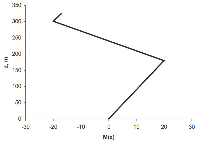
To illustrate the modal representation described in this section, we apply the above formulas to the case of radio wave propagation at wavelength λ = 9,1 cm in a surface based tropospheric duct created by M-profile, shown in Figure 3. Figure 4 shows the range dependence of the received signal strength at two elevations: 100 and 500 m.

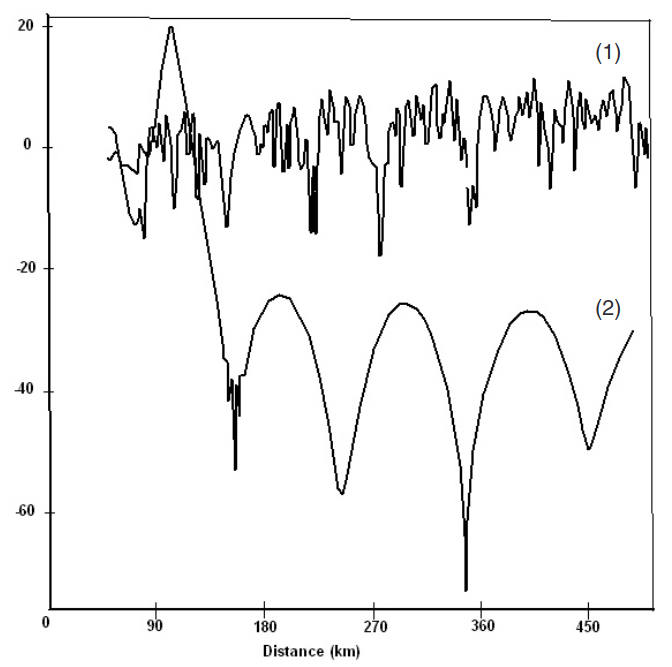
Graph: range dependence — Fig. 4 Range dependence of the received field at the wavelength 9,1 cm inside the duct (1) and above the duct (2)

The calculated signal strength clearly illustrates the multimode character of the field inside the duct at the height 100 m and the contribution of a few modes only for the receiving antenna above the duct (at 500 m). Figure 5 shows the impact on the radar coverage diagram at 10 GHz in case of the above tropospheric duct. It is observed that strong ducting mechanism allows for a target detection at the distances of several hundred miles.

Signal coverage — Fig. 5 Coverage diagram for 10 GHz source at 30,5 m for the surface-based duct formed by M-profile in Figure 3. The return path loss is 220 dB

Author

Olga Nesvetailova

Freelancer

Literature

Jensen, N.O., Lenshow, D.H. An observational investigation on penetrative convection. J.Atmos.Sci., 1978, 35(10), 1924–1933.;
Monin, A.S., Yaglom, A.M. Statistical Fluid Mechanics, Vol.1, MIT Press, Cambridge, MA, 1971, p. 769.;
Gossard, E.E. Clear weather meteorological effects on propagations at frequencies above 1 GHz, Radio Sci., 1981,16(5), 589–608.;
Tatarskii, V.I. The Effects of Turbulent Atmo- sphere on Wave Propagation, IPST, Jerusalem, 1971.;
Gavrilov, A.S., Ponomareva, S.M. Turbulence Structure in the Ground Level Layer of the Atmosphere. Collected Data, Meteorology Series, No.1, Research Institute for Meteorological Information, Obninsk (in Russian), 1984.;
Kukushkin, A.V., Freilikher, V.D. and Fuks, I.M. Over-the-horizon propagation of UHF radio waves above the sea , Radiophys. Quantum Electron. (translated from Russian), Consultant Bureau, New York , RPQEAC 30 (7), 1987, 597–620.;

Footnotes