Wave Excitation in Inhomogeneous Evaporation Ducts

Explore the phenomenon of wave excitation in evaporation ducts with a continuous spectrum, including the case of two trapped modes, and gain insights into the role of statistical inhomogeneity in shaping wave propagation patterns.

СодержаниеСвернуть

Excitation of Waves in a Continuous Spectrum in a Statistically Inhomogeneous Evaporation Duct
Evaporation Duct with Two Trapped Modes

In the absence of fluctuations in refractive index, δε, the signal strength in the shadow region above the evaporation duct is exponentially small because of the smallness of the “sub-barrier leakage” of the trapped modes.

Excitation of Waves in a Continuous Spectrum in a Statistically Inhomogeneous Evaporation Duct

The contribution of the waves of the continuous spectrum, initially excited by the transmitter, can be neglected because of the diffraction attenuation in the shadow region. The scattering of the waveguide trapped modes by random non-uniformities of the refractive index gives rise to incoherent exchange of energy between trapped modes and excitation of waves in the continuous spectrum. In addition, the initially excited waves of the continuous spectrum may reach beyond the horizon due to a scattering in the upper layers of the troposphere (Booker–Gordon’s single scattering mechanism). In this section, we study the contribution of the waves of the continuous spectrum, whose source is a waveguide mode, to the intensity of the field, i. e. the mechanism of the excitation of waves of the continuous spectrum by trapped modes of the evaporation duct scattered on the imhomogeneities in the refractive index.

Recalling the equations for the coherence function from the previous section, we concentrate on investigation of the spectral amplitude of the component of the coherence function related to a continuous spectrum:

{\tilde{g}}_{c} (x, E_{1}, E_{2}, p, γ) = \frac{1}{2 π} \int_{0}^{\infty} d z_{1} \int_{0}^{\infty} d z_{2} \int_{- \infty}^{\infty} d Y \cdot Γ (x, Y, γ, z_{1}, z_{2}) Ψ_{E_{1}}^{*} (z_{1}) Ψ_{E_{2}} (z_{1}) e x p (j p Y) E q . 1

As is well known, in the presence of random fluctuations of the refractive index, δε, the coherent component of the waves of the continuous spectrum attenuates with distance due to incoherent multiple scattering. The decrement of attenuation in the coherent component is given by:

γ_{c} = \frac{π k^{2}}{2} \int d^{2} {\vec{κ}}_{⊥} Φ_{ε} (0, {\vec{κ}}_{⊥}) E q . 2

where

Φ_{ε} (0, {\vec{κ}}_{⊥})

is the spectrum density of the fluctuations in δε. As observed in Understanding Parabolic Approximation in Wave Propagation: Analytical Methods and Applications“Green Function for a Parabolic Equation in a Stratified Medium”, in the case of free-space propagation with random irregularities of δε, the attenuation of the coherent component in the field intensity is completely compensated by the inflow of the incoherently scattered field from other directions, and the total intensity of the wave field does not reveal exponential attenuation. Since the propagation above the evaporation duct is free-space-like we may use the above argument in support of neglecting multiple scattering of the wave of the continuous spectrum in a space above the evaporation duct.

However, the effect of multiple scattering of the wave of the continuous spectrum can obviously be neglected if we demand a smallness of the attenuation of the coherent component of the CS spectrum wave, i. e., γ_c, x_a ≪ 1, over the path x_a of the wave from the point where scattering of the wave guide mode into the CS wave occurred up to the point of observation. Evaluating the maximum value of the distancex_a as

x_{a m a x} = \sqrt{2 a z},

where z is the height of the observation point, we obtain the limitation

z ≪ {(2 a γ_{c}^{2})}^{- 1} .

In the case of Kolmogorov’s turbulence:

γ_{c} = 2, 66 k^{2} C_{n}^{2} L_{0}^{5 / 3} .

Assuming

C_{n}^{2} = 10^{- 15} c m^{- 2 / 3}

, L₀ = 10⁴ cm, k = 2 cm^–1, we obtain the result that the maximum heights under consideration should not exceed the value z_max ~ 10³ m. Thus, the approximation in which the estimate is obtained below for the waves of the continuous spectrum is applicable for altitudes of the receiving point z satisfying the inequality z ≤ z_max.

Let us study the intensity of the field of the waves of the continuous spectrum:

I_{c} (x, z) = Γ (x, \vec{ρ}, \vec{ρ}), \vec{ρ} = \{0, z\},

setting the y-coordinates of the receiving and transmitting antennas to zero. Then, integrating Coherence Function in a Random and Non-uniform AtmosphereEquation and employing Coherence Function in a Random and Non-uniform Atmospherethe expression for the component of the coherence function associated with waves of the discrete spectrum, Γ_d, we obtain:

I_{c} (x, z) = \frac{k a^{2}}{16 x} {|ϕ_{d} (z_{0})|}^{2} e x p (- γ_{d} x) \cdot \int_{0}^{x} d x^{'} \int_{- \infty}^{\infty} d q \int_{Q < - |q| / 2} d Q B (q, Q) Ψ_{Q + q / 2} (z) Ψ_{Q - q / 2}^{*} (z) e x p (j \frac{q x^{'}}{2 k} + γ_{d} x^{'}) E q . 3

where we have introduced q = E₁-E₂, Q = (1/2)(E₁+E₂):

B (q, Q) = \int_{- \infty} d κ_{γ} \int_{- \infty} d κ_{z} Φ_{ε} (0, κ_{γ}, κ_{z}) \cdot \int_{0}^{\infty} d z_{1} \int_{0}^{\infty} d z_{2} Ψ_{Q + q / 2}^{*} (z_{1}) Ψ_{Q - q / 2} (z_{2}) ϕ_{d} (z_{1}) ϕ_{d}^{*} (z_{2}) e x p (j κ_{z} (z_{1} - z_{2})) . E q . 4

The integral B(q, Q) determines the coupling between the waves of the discrete and continuous spectra due to the scattering on the inhomogeneities of δε. The major contribution to B(q, Q) comes from the spectral components of δε with the wavenumbers:

|κ_{z}| > μ = {(- d U / d z)}^{1 / 3}

with z < Z_s and the region of the altitudes z_1,2 in the neighbourhood of the turning point z_d of the mode of the discrete spectrum, where U(z_d) = E_d. We use the WKB approximation for the waves of the continuous spectrum and the Airy function representation for the waveguide mode in the vicinity of the turning point:

Ψ_{E} (z) = \sqrt{\frac{2}{π}} {[U (z) - E]}^{- 1 / 4} e x p (- j \frac{3 π}{4}) \sin (\int_{0}^{z} d z^{'} \sqrt{U (z^{'}) - E}), E q . 5

ϕ_{d} (z) = \frac{1}{N_{d}} ν (μ (z - z_{d})), N_{d} = \int_{0}^{\infty} d z {|ϕ_{d} (z)|}^{2} .

The spatial spectrum of the fluctuations in the refractive index we define in the form (Atmospheric Boundary Layer and Basics of the Propagation Mechanismsin this equation) for the case of turbulent fluctuations δε isotropic in the (x, y)-plane:

Φ_{ε} (\vec{κ}) = 0, 033 C_{| |}^{2} α {(κ_{| |}^{2} + α^{2} κ_{z}^{2})}^{- 11 / 6} E q . 6

we substitute into Eqs. (4) and (5) the integral representation of the Airy function:

ν (t) = \frac{1}{2 \sqrt{π}} \int_{- \infty}^{\infty} d ξ e x p (j \frac{ξ^{3}}{3} + j ξ t)

and require the inequalities:

|κ_{z}| > μ a n d 2 \sqrt{E_{d}} \frac{m}{k} ≫ 1 E q . 7

to hold, which is necessary for the entire scheme of the solution obtained in Spectrum of Normal Waves in an Evaporation Duct“Detailed Wave Spectrum Analysis in Evaporation Ducts”. The meaning of inequality (7) is that we do not take into account the scattering of the leaky modes, assuming that the waveguide field is composed only of trapped (non-attenuated) modes. The B(q, Q) can then be truncated to:

B (q, Q) = C_{ε}^{2} α^{- 5 / 3} \cdot \{\begin{cases} 0, 089 \frac{\sin [q Λ_{d} (Q)]}{q N_{d}^{2} {(E_{d} - Q)}^{4 / 3}}, \frac{∆ κ}{κ_{d}} ≪ 1 \\ 0, 053 \frac{\cos [q Λ_{d} (Q)]}{μ^{3} N_{d}^{2} {(E_{d} - Q)}^{5 / 6}}, \frac{∆ κ}{κ_{d}} ≫ 1 \end{cases}) E q . 8

where:

Λ_{d} = \frac{1}{2} \int_{0}^{z_{d}} d z^{'} \sqrt{U (z^{'}) - Q}, κ_{d} = \sqrt{q_{d} - Q}, ∆ κ = \sqrt{U (0) - Q} - \sqrt{E_{d} - Q} E q . 9

Parameter κ_d determines the Bragg scattering angle θ_s from the waveguide mode into the wave of the continuous spectrum with energy Q at the height of the turning point z = z_d, i. e., 2 sin θ_s/2 = κ_d/k. The parameter Δk is a difference between the magnitude of the scattering angle at the surface z = 0 and at the altitude of the turn-ing point z = z_d. Thus the inequality Δκ/κ_d ≪ 1 requires that the change in the scattering angle owing to refraction in the scattering volume, i. e. in the region of the mode’s localization, be much smaller than the scattering angle itself at the altitude z_d.

The relationship between the characteristic “energy” Q and the sliding angle θ of the wave front of the wave of the continuous spectrum relative to the surface z = Z_s is given by the equation Q = -k²/m² tan²θ. The parameter Λ_d(Q) determines the distance along x traversed by the wave of the continuous spectrum with “energy” Q as it propagates from z = 0 to z = zd. Thus, B(q, Q) defines the angular distribution of the scattered field, i. e., the scattering function in the “directions” E1, E2.

To calculate the intensity of the field l_c(x, z) we employ the WKB approximation (4) and (7) in Eq. (2). We leave aside the constant terms for later and concentrate on the integration in Eq. (2). The integration over the “energy” difference q leads to the appearance of terms that place the limits on the region of the distances x^′ from which the scattered field is collected in the receiving antenna. With

\sqrt{U (0)} - \sqrt{q_{d}} / \sqrt{q_{d}} ≪ 1

we obtain:

I_{c} (x, z) ~ \int_{- \infty}^{0} d Q {(q_{d} - Q)}^{- 4 / 3} {(U (z) - Q)}^{- 1 / 2} \int_{0}^{x} d x^{'} e x p (γ_{d} x^{'}) \cdot \{\frac{1}{2} θ (Λ_{d} + Λ - \frac{x^{'}}{k}) - \frac{1}{2} θ (Λ_{d} - Λ - \frac{x^{'}}{k}) - θ (Λ_{d} - \frac{x^{'}}{k}) \cos (2 \int_{0}^{z} d z^{'} \sqrt{U (z^{'}) - Q})\} E q . 10

and for

\frac{\sqrt{U (0)} - \sqrt{q_{d}}}{\sqrt{q_{d}}} ≫ 1 :

I_{c} (x, z) ~ \int_{- \infty}^{0} d Q {(q_{d} - Q)}^{- 5 / 6} {(U (z) - Q)}^{- 1 / 2} \int_{0}^{x} d x^{'} e x p (γ_{d} x^{'}) \cdot \{\frac{1}{2} δ (\frac{x^{'}}{k} + Λ_{d} - Λ) + \frac{1}{2} δ (\frac{x^{'}}{k} - Λ_{d} + Λ) + \frac{1}{2} δ (\frac{x^{'}}{k} - Λ_{d} - Λ) - δ (\frac{x^{'}}{k} - Λ_{d}) \cos (2 \int_{0}^{z} d z^{'} \sqrt{U (z^{'}) - Q})\} E q . 11

where:

θ (x) = \{\begin{matrix} 1, x > 0 \\ 1 / 2, x = 0 \\ 0, x < 0 \end{matrix}\}

and:

Λ = Λ (Q, z) = \frac{1}{2} \int_{0}^{z} d z^{'} \sqrt{U (z^{'}) - Q} .

We introduce the dimensionless variables τ = -Qm²/k², τ_d = E_dm²/k², h = kz/m, β = m²γ_s/k and the modified profile U(h) = m²/k²U(z). We then require that the inequality:

k γ_{d} Λ_{d} (0) ≪ 1 E q . 12

holds. Since Λ_d(0) ≥ Λ_d(E_d), where kΛ_d(E_d) the length of the cycle of a waveguide mode and the contributing values of Q are limited by the inequality |Q| ≤ E_d, the condition (12) demands the smallness of the attenuation of the waveguide mode at the distance equal to its cycle. It may be noted that in the opposite case there is no waveguide mode structure to sustain scattering, the mode will be destroyed during one cycle.

Finally we obtain the intensity of the wave of the continuous spectrum normalized at the intensity of the free-space field:

J_{c} (x, z) = I_{c} (x, z) \frac{x^{2}}{a^{2}} = 0, 078 k^{- 5 / 3} x C_{ε | |}^{2} α^{- 5 / 3} m^{11 / 3} (\frac{{|ϕ_{d} (z_{0})|}^{2}}{N_{d}^{2}}) \cdot K (h) e x p (- γ_{d} x) E q . 13

and the function K(h), which commands that the height distribution of the scattered field is given by two equations obtained from Eqs. (10) and (11). With

\sqrt{U (0)} - \sqrt{τ_{d}} / \sqrt{τ_{d}} ≪ 1 :

K (h) = \int_{0}^{\infty} d τ {(τ_{d} + τ)}^{- 4 / 3} {(U (h) + τ)}^{- 1 / 2} Λ_{d} (τ) \cdot \{e x p (β Λ (τ, h)) - \cos (2 \int_{0}^{h} d h^{'} \sqrt{U (h^{'}) + τ})\}, E q . 14

and for

\sqrt{U (0)} - \sqrt{τ_{d}} / \sqrt{τ_{d}} ≫ 1 :

K (h) = {π {[- \frac{d U}{d h}]}^{- 2 / 3}}_{h = h_{d}} \int_{0}^{\infty} d τ {(τ_{d} + τ)}^{- 5 / 6} {(U (h) + τ)}^{- 1 / 2} \cdot \{e x p (β Λ (τ, h)) - \cos (2 \int_{0}^{h} d h^{'} \sqrt{U (h^{'}) + τ})\} . E q . 15

We shall now study the total field in the shadow region as being the result of composition of the waves of the discrete and continuous spectra excited due to the random scattering of the waveguide modes. For the intensity of the waveguide mode the relation below follows:

J_{d} = \frac{x}{8 π k {|N_{d}|}^{4}} {|ϕ_{d} (z_{0})|}^{2} {|ϕ_{d} (z)|}^{2} e x p (- γ_{d} x) . E q . 16

We define the total intensity as:

J_{t o t} = J_{d} + J_{c} = \frac{x}{8 π k {|N_{d}|}^{2}} {|ϕ_{d} (z_{0})|}^{2} e x p (- γ_{d} x) S (z) E q . 17

where:

S (z) = \frac{{|ϕ_{d} (z)|}^{2}}{N_{d}^{2}} + 0, 139 k^{- 2 / 3} C_{ε}^{2} α^{- 5 / 3} m^{11 / 3} K (z) . E q . 18

The function S(z) determines the height distribution of the total intensity of the field. We examine the behavior of the function S(z) in the case of a bilinear dependence of U(z). We assume the following values for the parameters of the problem:

k = 2 cm^–1;
a = 8 500 km;
Z_s = 11 m;
Δε_M = ε_M(0)-ε_M(Z_s) = 5,8·10⁶.

The modified profile U(h) can be defined as:

U (h) = \{\begin{cases} μ_{1}^{3} (H_{s} - h), h \geq H_{s} \\ h - H_{s}, h > H_{s} \end{cases}) E q . 19

where:

H_s = kZ_s/m = 2,42;
$μ_{1}^{3} = m^{2} ∆ ε_{M} / H_{s} = 2;$
$τ_{d} = U (0) - μ_{1}^{2} τ_{1} = 1;$
U(0) = m²Δε_M = 4,34;
τ₁ = 2,338.

Consider the height dependence of the waveguide mode, i. e., the first term in S(z). Thus far in the analysis of the waveguide field we have neglected the leakage of the trapped waves of the discrete spectrum through the potential barrier. The attenuation caused by the effect of the leakage is accounted for in the imaginary part of E_d, which can be written as:

δ_{d} = Im E_{d} = \frac{μ^{2} μ_{1}^{2}}{4 \sqrt{τ_{1}}} e x p \{- \frac{4}{3} τ_{d}^{3 / 2} \frac{1 + μ_{1}^{3}}{μ_{1}^{3}}\} . E q . 20

Sub-barrier leakage has virtually no effect on the height structure of the trapped mode inside the waveguide channel for h < H_s, where:

ϕ_{d} (h) = \frac{1}{N_{d}} ν (\frac{τ_{d}}{μ_{1}^{2}} - μ (H_{s} - h)) . E q . 21

Outside the waveguide channel the height structure of ϕ_d(h) corresponds to an outgoing wave with amplitude proportional to the leakage factor δ_d:

ϕ_{d} (h) = \frac{μ_{1}^{- 1 / 3}}{μ N_{d}} τ_{1}^{1 / 4} δ_{d}^{1 / 2} w_{1} (τ_{d} + j \frac{δ_{d}}{μ^{2}} - (h - H_{s})) . E q . 22

Examining the second term in S(z) given by Eq. (18), we can express the coefficient in front of K(z) in terms of the non-dimensional attenuation coefficient b using Coherence Function in a Random and Non-uniform AtmosphereEquation for γ_d from the previous section:

β = m^{2} γ_{d} / k = 0, 264 k^{- 2 / 3} C_{ε | |}^{2} α^{- 5 / 3} m^{11 / 3} μ_{1}^{- 5 / 9} .

Then for S(z) we obtain:

S (z) = \frac{{|ϕ_{d} (z)|}^{2}}{N_{d}^{2}} + 0, 492 μ_{1}^{5 / 9} β K (z) . E q . 23

In principle, in order to determine the coefficient β it is necessary to know the magnitude of the structure constant C_ε and the anisotropy parameter of the irregularities of the refractive index in the volume of the waveguide channel. In some cases when the radio signal strength is measured, the measured data may be deployed to estimate the height dependence of the received signal. In particular, when the magnitude of the field attenuation per unit length γ_x = dI/dx is known from the measured signal, then γ_d is related to γ_x via γ_x = 4,34γ_d, and given knowledge of the average M-profile we can construct a theoretical height structure of the field intensity S(z).

The γ_x magnitude for centimeter waves lies in the range γ_x = 0,2–0,5 dB km^–1. The corresponding limits for β are β = 0,207–0,52 for k = 2 cm^–1 and a = 8 500 km (normal refraction above the evaporation duct). Thus under real conditions the coefficient in front of K(z) in Coherence Function in a Random and Non-uniform AtmosphereEquation is of the order of unity and, consequently, the contribution of the waves of the continuous spectrum to S(z) can be significant.

Figure 1 shows the result of the calculation of the resulting height distribution 10 log S(h) based on Eq. (23) for β = 0,207 and β = 0,52 with U(h) given by Eq. (19) and its parameters defined above.

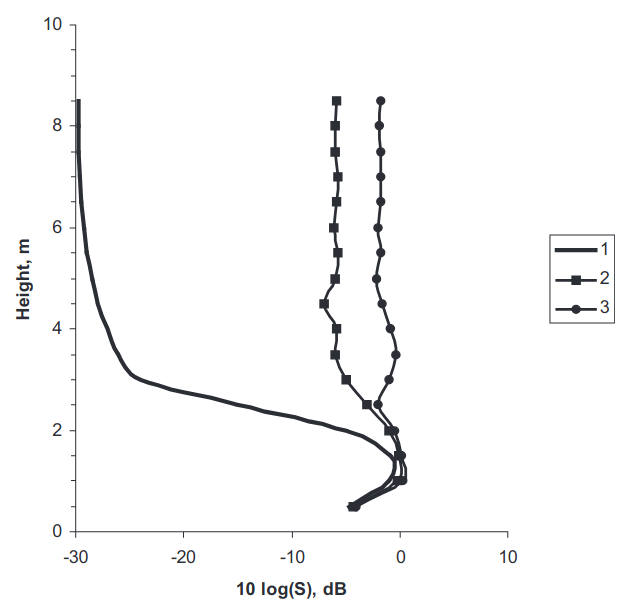
Fig. 1 Height structure of the wave field in the presence of an evaporation duct: f = 10 GHz, Curve 1, no scattering on inhomogeneities of the refractive index, curves 2 and 3, scattering is taken into account

The figure also shows the height dependence of the first term in Eq. (23), i. e., the contribution of the waves of the discrete spectrum alone. As observed from the figure, the intensity of the field above the turning height h_d (in this case h_d = 1,67) is a contribution from the waves of the continuous spectrum, i. e. second term in Eq. (23). Apparently, scattering on random fluctuations in the refractive index leads to a significant change in the height dependence of the signal strength; in the presence of random fluctuations de in the refractive index there is no sharp exponential decay in the average signal strength outside the duct and for sufficiently strong fluctuations the δε field outside the duct may increase to the order of magnitude of the field inside, thus revealing a rather smooth unpronounced height dependence compared to the case of deterministic duct propagation.

At relatively large altitudes, h = H_s ≫ τd, the function S(h) has the following asymptotic form:

S (h) ~ \frac{1}{4 \sqrt{h - H_{s} - τ_{d}}} e x p [- \frac{4}{3} τ_{d}^{3 / 2} \frac{μ_{1}^{3} + 1}{μ_{1}^{3}} + 2 \frac{δ_{d}}{μ^{2}} \sqrt{h - H_{s} - τ_{d}}] + \frac{1, 58 μ_{1}^{5 / 9} β}{τ_{d}^{1 / 3} \sqrt{h - H_{s}}} e x p (β \sqrt{h - H_{s}}) . E q . 24

Beginning with the altitudes

h_{1} = H_{s} + τ_{d} + \frac{μ^{4}}{2 δ_{d}^{2}}

and

h_{2} = H_{s} + \frac{1}{4 β^{2}},

the exponential growth predominates over the cylindrical divergence in either the first or second terms, respectively.

The exponential growth of those terms in Eq. (24) is due to the arrival of the waves from shorter distances x^′ < x, at which the field of the waveguide mode was exponentially large, compared with its value at distance x. The second term makes the main contribution in Eq. (24), since the exponential factor β exceeds the sub-barrier leakage factor δ by at least an order of magnitude.

As mentioned before, we ignored the scattering of the waves in the space above the waveguide. While, in principle, it should be taken into account for the sake of consistency, the qualitative character of the total field will not be expected to change drastically. We may assume however that additional scattering of the waves of the continuous spectrum in the space above the evaporation duct will smooth the exponential dependence of the scattered field in Eq. (24) for large altitudes. At the same time additional divergence of the waves due to a broadening of the angular spectrum can be compensated by the arrival of the scattered waves from the shadow region, i. e. from distances

x^{'} < x - a / m \sqrt{h - H_{s}} .

Evaporation Duct with Two Trapped Modes

Finally, we provide a closed form solution for the field intensity in the case when the evaporation duct can trap two modes. In this case the intensity in the two-mode waveguide is given by:

J (x, z, z_{0}) = 4 π x [I_{1} \cdot S_{1} + I_{2} \cdot S_{2}] E q . 25

where:

I_{1} (x) = A_{1} e^{λ_{1} x} + A_{2} e^{λ_{2} x},

I_{2} (x) = A_{3} e^{λ_{1} x} + A_{4} e^{λ_{2} x},

λ_{1, 2} = - \frac{Γ_{1} + Γ_{2}}{2} \pm \frac{1}{2} \sqrt{{(Γ_{2} - Γ_{1})}^{2} - 4 W_{12}},

A_{1} = - \frac{[I_{10} (λ_{2} + Γ_{2}) - W_{12} I_{20}]}{λ_{1} - λ_{2}},

A_{2} = - \frac{[I_{10} (λ_{1} + Γ_{1}) - W_{12} I_{20}]}{λ_{1} - λ_{2}},

A_{3} = - \frac{[I_{20} (λ_{2} + Γ_{2}) - W_{12} I_{10}]}{λ_{2} - λ_{1}},

A_{4} = - \frac{[I_{20} (λ_{1} + Γ_{1}) - W_{12} I_{10}]}{λ_{1} - λ_{2}},

Γ_{1} = 1, 603 \cdot A_{s}, Γ_{2} = 3, 98 \cdot A_{s}, W_{12} = 0, 316 \cdot A_{s}, and A_{s} = k^{- 2 / 3} C_{ε}^{2} α^{- 5 / 3} m^{11 / 3} .

Coefficients I_n0 = |χ_n(h₀)|² are the coefficients of the excitation of the mode with number n and function S_n(h) is a height distribution of the total intensity of the nth mode:

S_{n} (h) = {|χ_{n} (h)|}^{2} + 0, 492 Γ_{n} μ_{1}^{5 / 3} P_{n} (h) . E q . 26

The height gain function χ_n is given by:

χ_{n} (h) = \frac{\sqrt{μ_{1}}}{τ_{n}} ν (\frac{t_{n} - U (h)}{μ_{1}^{2}}), h < H_{s} E q . 27

χ_{n} (h) = δ^{1 / 2} w_{1} (\frac{t_{n} - U (h)}{μ_{2}^{2}}), h \geq H_{s}

where δ is the coefficient of penetration through the potential barrier into the space above the duct:

δ = \frac{μ_{1}}{4 τ_{n}} e x p [- \frac{4}{3} \frac{μ_{2}^{3} + μ_{1}^{3}}{μ_{1}^{3} μ_{2}^{3}} t_{n}^{3 / 2}], E q . 28

τ_{n} = {[\frac{3}{2} π (n - \frac{1}{4})]}^{2 / 3} .

The function P_n(h) is given by the integral:

P_{n} (h) = π / μ_{1}^{2} \int_{0}^{\infty} d s {(t_{n} + s)}^{- 5 / 6} {(U (s) + s)}^{- 1 / 2} [e^{Λ (s, h)} - \cos (2 Q (s, h))] E q . 29

where:

Q (s, h) = \frac{2}{3 μ_{1}^{3}} [{(U_{0} + s)}^{3 / 2} - {(U (h) + s)}^{3 / 2}], h < H_{s} E q . 30

Q (s, h) = \frac{2}{3} [\frac{1}{μ_{1}^{3}} {(U_{0} + s)}^{3 / 2} - \frac{μ_{1}^{3} + μ_{2}^{3}}{μ_{1}^{3} μ_{2}^{3}} + {(U (h) + s)}^{3 / 2}], h \geq H_{s}

Λ (s, h) = \frac{1}{μ_{1}^{3}} {(U_{0} + s)}^{1 / 2} - \frac{1}{μ_{1}^{3}} {(U (h) + s)}^{1 / 2}, h < H_{s} E q . 31

Λ (s, h) = \frac{1}{μ_{1}^{3}} {(U_{0} + s)}^{1 / 2} - \frac{μ_{1}^{3} + μ_{2}^{3}}{μ_{1}^{3} μ_{2}^{3}} + {(U (h) + s)}^{1 / 2}, h \geq H_{s} .

It should be noted that the above formulas actually represent the incoherent sum of two trapped modes. Under very moderate assumptions for the intensity of the atmospheric turbulent fluctuations (as in Figures 2 and 3 below) the interference term in the coherence function may be neglected since phase fluctuations in this case are strong enough to make the above approximation valid.

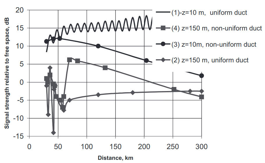
Atmospheric turbulent fluctuation — Fig. 2 Range dependence of the signal strength at 10 GHz in the presence of an evaporation duct with two trapped modes

On Figure 2 the transmitter antenna is mounted at 10 m above the sea surface. Curves (1) and (2) correspond to the range dependence of the received field strength for the receiving antennas at the heights inside (1) and outside (2) the duct for the case of a uniform duct in the absence of random fluctuations in the refractive index. Curves (3) and (4) correspond to the same antenna elevations for a non-uniform duct with random and anisotropic fluctuations of the refractive index:

C_{ε}^{2} = 10^{- 14} c m^{- 2 / 3}, α = 0, 1 .

Signal strength — Fig. 3 Height-gain dependence of the signal strength at 10 GHz in the presence of an evaporation duct with two trapped modes at 100 km from the transmitter

On Figure 3 The transmitter antenna is mounted at 10 m above the sea surface. Curve (1) shows the received field versus the height in the absence of random fluctuations in the refractive index. Curve (2) is a height-gain dependence for a non-uniform duct with random and anisotropic fluctuations of the refractive index:

C_{ε}^{2} = 10^{- 14} c m^{- 2 / 3}, α = 0, 1 .

To illustrate the effect of scattering on random fluctuations in a two-mode evaporation duct we calculated the signal strength at frequency 10 GHz in the evaporation duct with parameters Z_s = 15 m and ΔM = 5 N-units. Figure 2 shows a range dependence of the signal strength in the absence and presence of the fluctuations in the refractive index. As observed from the figure, at a height 10 m inside the duct the composition of the two trapped modes produces an interference pattern, creating fades. The second curve shows the range dependence at the height 150 m where the second trapped mode is dominant and therefore no interference pattern is observed. The height gain pattern in this case is typical for one that follows from the model of the evaporation duct, namely, revealing the maximum of the signal strength inside the duct, Figure 3. In the presence of fluctuations we observe significant attenuation of the field with distance as well as considerable changes in the height gain distribution, namely, the height structure becomes largely uniform.

In the range of frequencies from 3 GHz to 20 GHz the evaporation duct in most cases can support only a few trapped modes. The calculation of the field strength for a finite number of modes can be performed in a way similar to that described in this section. The surface-based and elevated duct created by an advection mechanism and normally associated with strong elevated inversion of temperature may trap a hundred modes and the above approach is inefficient. In that case other methods based on the application of diffusion theory for a parabolic equation can be employed to solve the problem of scattering in a multimode waveguide.

Author

Olga Nesvetailova

Freelancer

Literature

Jensen, N.O., Lenshow, D.H. An observational investigation on penetrative convection. J.Atmos.Sci., 1978, 35(10), 1924–1933.;
Monin, A.S., Yaglom, A.M. Statistical Fluid Mechanics, Vol.1, MIT Press, Cambridge, MA, 1971, p. 769.;
Gossard, E.E. Clear weather meteorological effects on propagations at frequencies above 1 GHz, Radio Sci., 1981,16(5), 589–608.;
Tatarskii, V.I. The Effects of Turbulent Atmo- sphere on Wave Propagation, IPST, Jerusalem, 1971.;
Gavrilov, A.S., Ponomareva, S.M. Turbulence Structure in the Ground Level Layer of the Atmosphere. Collected Data, Meteorology Series, No.1, Research Institute for Meteorological Information, Obninsk (in Russian), 1984.;
Kukushkin, A.V., Freilikher, V.D. and Fuks, I.M. Over-the-horizon propagation of UHF radio waves above the sea , Radiophys. Quantum Electron. (translated from Russian), Consultant Bureau, New York , RPQEAC 30 (7), 1987, 597–620.;

Footnotes