Explore the scattering mechanism of over-horizon UHF propagation through a detailed analysis of basic equations, perturbation theory for field moment calculations, and the interaction of diffracted fields with turbulent refractive index fluctuations.
As discussed in Atmospheric Boundary Layer and Basics of the Propagation Mechanisms“Atmospheric Boundary Layer and Key Propagation Mechanisms”, the analytical study of wave propagation through a turbulent troposphere is complicated due to the high dynamic range of the turbulent fluctuations of the refractive index as well as the presence of the boundary surface.
In UHF Propagation in an Evaporation Duct“Exploring UHF Propagation in Evaporation Ducts” we studied the impact of the random component of the dielectric permittivity of the troposphere on UHF propagation in an evaporation duct. It was shown that wave scattering on random inhomogeneities of the refractive index leads to a non-coherent redistribution of the energy between the waveguide modes, the loss of coherence results in additional attenuation of the trapped modes. Using the language of quantum mechanics, we have found the perturbations to the eigenvalues of the discrete spectrum of the localised states. The results obtained in UHF Propagation in an Evaporation Duct“Exploring UHF Propagation in Evaporation Ducts” are valid at distances from the source, on the one hand, long enough to filter all leaked modes and, on the other hand, not too long so that the scattering in the upper layers of the troposphere can be neglected in comparison with the field carried by the trapped modes.
In the absence of tropospheric ducts it is sometimes convenient to solve the transport equations for the coherence function in the continuum spectrum. Such a solution has been obtained for multiple wave scattering in a random medium (uniform on average) over the flat boundary surface. The results demonstrated that anisotropic inhomogeneities of the refractive index may have a significant impact on the signal level. The multiple scattering in the case of strong anisotropy was studied in Refs, where the following was shown:
Similar results were obtained, where the authors derived integro-differential equations for the field moments which account for diffraction on the random inhomogeneties and variations in the trength of scattering with small scattering angles. The important result is that the Markov approximation is not applicable with extremely large parameters of anisotropy. In such cases the two-scale model may provide a sufficient tool for analysis.
In this article we suggest a technique for calculating the coherent signal component, with allowance for both diffraction by the earth and wave scattering on random inhomogeneities of the refractive index. Theoretically, the coherent component is defined as the complex amplitude averaged over a statistical ensemble of realisation. If the ergodicity and locally frozen hypotheses hold, the ensemble averaging is equivalent to such over an infinitely long interval. For practical purposes, however, the component coherent over a finite interval of time is of interest. According to data provided in Refs, in about 60 % of experiments performed on trans-horizon links up to 300 km in length, the received amplitude distribution is different from Rayleigh law. This difference is ascribed to the effect of the coherent component. Therefore, it seems necessary to analyse all the factors influencing the coherent component, its range and wavelength dependences, etc.
The approach can be formulated in the following way. For the electromagnetic field component, coherent over time T, we derive, using the Markov approximation, a parabolic-type equation allowing for the additional decay of the coherent signal due to scattering on small-scale fluctuations of the refractive index. Further, we analyse the possibility of replacing in the equation the average (over time T) dielectric constant, which is a “slowly varying” random function of all three variables, with a random function depending on a single coordinate, i. e. height over the interface. Through this procedure, the problem of wave propagation through a three-dimensional random medium is reduced to that for a random stratified medium. The field component averaged over time T can be represented in this approach as a normal wave (i. e. modal) series with random propagation constants and height gain functions for each mode. These are determined with the aid of the perturbation technique formulated in Wave Field Fluctuations in Random Media over a Boundary Interface“Understanding Wave Field Fluctuations in Random Media”, in which the unperturbed refractive index profile is that averaged over the ensemble of the realizations, and the random stratification due to large-scale anisotropic inhomogeneities is considered as a perturbation. The approach permits one to obtain closed-form expressions for statistical moments of any order and analyse the correlation between the signal levels and the turbulent troposphere.
It seems noteworthy that at decimetre wavelength the attenuation rate of the coherent component (T ≤ 1 min) is not normally very high, hence at links about 200 km long the coherent intensity practically coincides with the whole decimetre signal. The basic observation is that the approach suggested in this article is better suited to wave propagation effects at frequencies below 1 GHz, where the effect of the ducting is also week.
Basic Equations
Consider a vertically polarized field whose attenuation function (Understanding Parabolic Approximation in Wave Propagation: Analytical Methods and Applicationssee this equation) is governed by the parabolic equation:
where εM(x, γ, z) = ε(x, γ, z)+2z/2.
As is known, scattering on the fluctuation in the dielectric permittivity brings about additionnal attenuation of the coherent component of the field which can be described by the factor e-γx. In the Markov process approximation, the decrement of attenuation γ is given by:
and transforming Eq. (1) to the integral equation form we obtain:
provided that the wave propagation can be regarded as a Markovian process, i. e. the conditions below are met:
Here:
The attenuation rate γT averaged over the fluctuations in Eq. (3) is given by the relation:
and:
νγ can be estimated as a mean value of the horizontal transfer velocity:
We can assume, for further estimates, that κzT ≈ (σνzT)-1. The conditions (4) were obtained in Refs for a spatially uniform field of δε. The inequalities (4) impose some limitations to an averaging time T, since under “frozen” turbulence conditions L|| = ν||T, Lz = σνzT, therefore instead of Eq. (4) we obtain:
and:
for “locally uniform” turbulence.
we can present WT (x, γ, z) as:
where:
Estimating the integral in Eq. (12) we will first assume εT(z) to correspond to the standard tropospheric refraction, i. e. εT(z) = 1+2 z/2. Explicit expressions for the values involved in Eq. (15) are:
With:
the mean-square log-amplitude fluctuations are:
we see that the principal inequality (18a) can hold at x ≤ 103 km.
Perturbation Theory: Calculation of Field Moments
assuming specifically:
To determine the propagation constants and height gain functions, we will make use of the perturbation theory described in Wave Field Fluctuations in Random Media over a Boundary Interface“Understanding Wave Field Fluctuations in Random Media”. Representing q and χ as:
where q0 and χ0 are governed by the unperturbed Eq. (11) with εT(z) = ε0(z). We can obtain the random correction term δq and ς(z) in the form:
Now we single out of WT(x, γ, z; z0) the value W0, i. e. the solution to Eq. (11) with εT(z) = ε0(z), to obtain:
The factor WT (x, γ, z; z0) is a random function of a “slow” time t > T. Within each realization of the signal, the factor WT is the coherent component of the total signal received during the “short” intervals t ≤ T. During the “long” time-interval t ≫ T, the factor WT undergoes relatively slow random variations owing to changes of realisation of εT. The part of WT fluctuating at the change of realisations Δε(z) is given by the exponent of Eq. (25).
We can specify the intensity J0 of the coherent component WT (x, γ, z; z0) given ε0(z) in the form (20):
As can be observed from Eqs. (23) to (25), the random value WT should be distributed log-normally, in view of the central limiting theorem. Note that similar distributions are actually observed in the experiment. For instance, the integral distribution of the amplitude measured over 1 to 5 min intervals reveals log-normal statistics.
To simplify further the derivations, we will assume the receiver and transmitter heights to be equal, i. e. z = z0, and consider the intensity JT of the coherent (over time T) signal component averaged over the statistical ensemble, viz.
Further calculations are straightforward but cumbersome. As a specific example, consider one of the correlators involved in Eq. (27):
The corresponding terms δq can be expressed via the Fourier transform of Δε(z), viz.
where the function V(κ) is given by:
It has the meaning of the scattering coefficient from the first mode back to itself again, due to inhomogeneities Δε(z) of the scale-size l = 2π/κ.
According to the inequality (14), the major contribution to the random component of the vertically stratified Δε(z) is given by sufficiently large inhomogeneities with κ = κz ≪ k/m. For this case V(κ) can be represented by an asymptotic expansion:
Defining the spectral density of the fluctuations as:
The range of validity of Eq. (35) is dictated, according to the perturbation method employed, by the demand that the second-order correction to WT(x, z; z0) be small.
Analyzing Eqs. (27) and (29) we find that the corrections to the propagation constants take the major role in the second-order corrections overall, and these can be evaluated as:
and a = 8 500 km. Range dependences J0 are also shown for comparison. As can be seen from Figure 1 and from Eq. (35), the presence of random gradients dεT/dz ~ σΔε/Lz in the refractive index results in a sharp increase in the signal strength. This can be regarded as a kind of “trapping” or localization of the radiated field near the earth’s surface, however, in this case it is of a random nature.
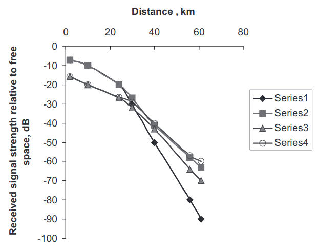
- Received field strength at frequency 3 GHz in the absence of fluctuations in the refractivity ();
- Received field strength at frequency 3 GHz, in the presence of fluctuations in the refractivity
- Received field strength at frequency 1 GHz in the absence of fluctuations in the refractivity();
- Received field strength at frequency 1 GHz, in the presence of fluctuations in the refractivity
Making use of Eqs. (25), (27) and (35), we can evaluate the square of the standard of the intensity fluctuations, viz.
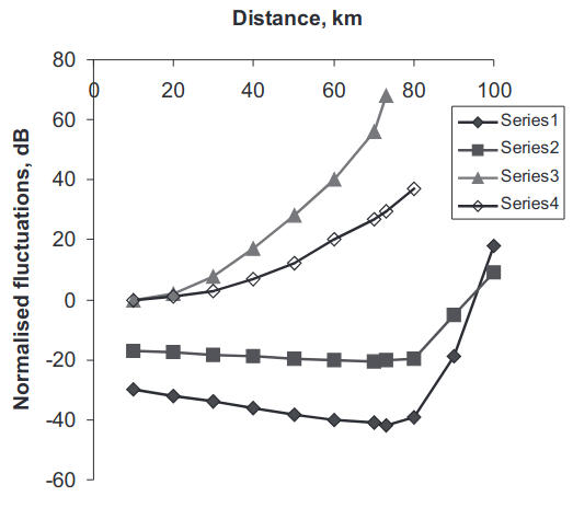
- Fluctuation standardat frequency 3 GHz;
- Fluctuation standardat frequency 1 GHz;
- Variation indexfrequency 3 GHz;
- Variation indexat frequency 1 GHz.
We believe that Eqs. (35) and (38) can provide an explanation for the increase in the fading depth which is observed experimentally with increase in the mean levels of the signal. According to the field measurements, the fading depth increases with the path length up to ~200 km, such behavior is also in agreement with the theoretical result provided by Eq. (38). The above theory, developed in this section, introduces a two-scale model of fluctuations in the refractive index: small-scale fluctuations treated as a Kolmogorov turbulence and large-scale fluctuations Δε which are treated as a random stratification Δε(z).
Yet, as can be seen from the above theory, the random component of Δε(z) can play the dominant part in cases where the average profile does not reveal a strong near-surface inversion, like an evaporation duct or for frequencies significantly below 10 GHz when an evaporation duct, even if present, is normally insufficient for the ducting mechanism at these frequencies.
Scattering of a Diffracted Field on the Turbulent Fluctuations in the Refractive Index
Long-range tropospheric propagation due to re-emission of the energy of electromagnetic waves by inhomogeneities of the refractive index has been known since the 1940s. The simple mechanism of the single scattering was first developed by Booker and Gordon and then updated taking into account the Kolmogorov the- ory of the turbulent spectrum of fluctuations in the refractive index. The theory of single scattering was proposed to explain the phenomenon of the long-range propagation in the absence of super-refractive anomalies in the refractive index profiles. It takes into account scattering by inhomogeneities located in the region formed by the intersection of the directional diagrams of the receiving and transmitting antennas, as shown in Figure 4.
According to Refs, the mean intensity Js of the scattered field Is normalised on the intensity in a free space IFS is expressed as follows:
where V is the effective scattering volume and R is the distance between the receiver and transmitter, and σ0 is the effective scattering cross-section.
The effective scattering cross-section σ0 from a unit volume to a unit solid angle is given by:
For the inertial interval of the turbulence spectrum s0 is determined by the relation:
where Cε is a structure constant, Understanding Parabolic Approximation in Wave Propagation: Analytical Methods and Applications“Parabolic Approximation to the Wave Propagation”.
The above Booker–Gordon theory provides rather good estimates of the signal strength of the scattered field as well as describing the range dependence of the receiving signal strength. However, there are several factors which, in the majority of observations, are not in agreement with the theory of single scattering, for example, the dependence on wavelength, elevation angle, and the cumulative distribution of the scattered field.
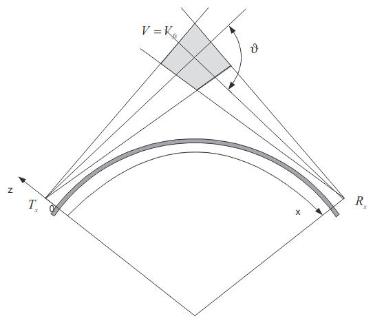
In this section we attempt to estimate the intensity of the signal over the horizon due to scattering of the waves in the volume located in the geometric shadow relative to both the transmitter and receiver, as shown in Figure 5.
Consider the case of normal refraction, in which the modified dielectric constant of the troposphere εM(x, γ, z) = ε0(z) + δε(x, γ, z), ε0 = 1 + 2z/a. Here δε(x, γ, z) is a random component of the dielectric permittivity, <δε> = 0.
We shall define the mean intensity Js of the scattered field normalised at an intensity in a free space via the attenuation factor W:
The attenuation factor can be represented in the form W = W0+W1, where W0 is the solution of the equation:
and W1 is defined in the Born approximation by the expression:
Later we will set x0 = 0 and γ = γ0 = 0.
We also restrict the integration volume for discussion of the scattering of a diffracted field in the shadow region by the inequalities:
Here:
We note that the Booker–Gordon theory takes account of scattering only in the radiated region bounded by the inequality:
which is represented in shadow region in the series of normal waves, Understanding Parabolic Approximation in Wave Propagation: Analytical Methods and Applications“Parabolic Approximation to the Wave Propagation”:
where qn is a complex propagation constant:
The height-gain functions χn(z) satisfy the equation:
and boundary conditions:
For the case of normal refraction χn(z) can be represented in terms of the Airy function, χn(z) = w1(tn-μz), where μ = k/m and tn = qn/μ2.
We shall substitute Eqs. (47) and (48) into Eq. (44) and take into account in the double summation over the modes only diagonal terms which do not oscillate with distance. Integrating in Eq. (44) over dy and assuming statistical uniformity of the fluctuations in the refractive index and their isotropy in the x-, γ-planes, we can obtain the equation:
is a factor describing the dependence of the mean intensity of the scattered field on altitude and x1 = x-Δx-Δx0.
The function Vn(κz, x′) in Eq. (52) has the meaning of a coefficient of re-scattering from the nth mode into the nth mode by inhomogeneities with the scale lz = 2π/κz and is defined by:
With:
the major contribution to integral (53) comes from the altitude’s interval 0 < z < mτn/2k. The upper limit in Eq. (53) in this case can be replaced by infinity by means of introducing a smooth limiting function which compensates the growth of:
Let us introduce such a function in the form of exponent exp(-βz). After transition to non-dimensional variables α = β m/k, ς = kz/m and q = κzm/k we can deform the contour of integration over ς in Vn(κz, x) into a ray with arg ς = π/3. With α ≠ 0 we can neglect the contribution from integration over the arc of infinite radius, and for Vn(κz, x) we then obtain:
where:
is the Airy function. We can further put parameter α = 0 and expand the exponent into a series over powers of q*ς:
where:
The recurrent formulas for integrals (56) are provided in the Airy Functions – Comprehensive Guide“In-Depth Exploration of Airy Functions and Their Applications”.
With |q|τn ≪ 1, we can retain only the first term in series (55). Taking into account that ν(-τn) = 0, we obtain the asymptotic expression:
when:
the stationary point of the integrand in Eq. (53):
When κz > 2kx/a, the upper limit of integration makes the main contribution to the integral Vn(κz, x):
This equation corresponds to non-resonant scattering by inhomogeneities with scales lz < πa/kx.
where:
This spectrum takes into account the finite external scales along the vertical (Lz) axis and horizontal plane (L||) and the anisotropy of the inhomogeneities α = Lz/L|| ≠ 1.
Taking then account of the fact that for x ≫ a/mτn (for f ~ 10 GHz, a/mτn ~ 10 km) small-scale inhomogeneties with κz ≫ k/mτn make the main contribution to the scattering, and bearing in mind that mτn ≫ 1, we obtain for the intensity of the scattered field Js the following expression:
where:
We have taken into account the contribution of the first mode with n = 1, the scattering of the other modes can be estimated similarly, however, the contribution of the modes with higher indices n decays as n–2.
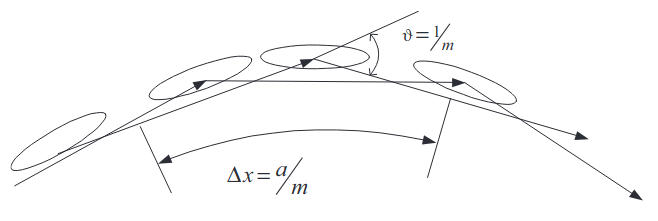
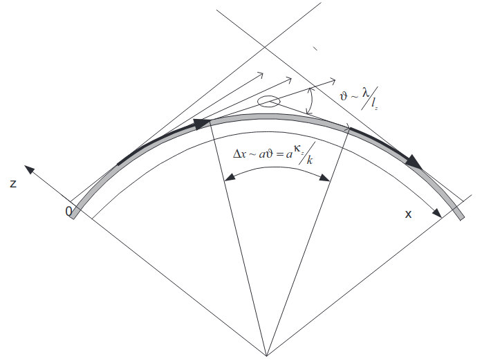
The contribution of the large-scale inhomogeneities to the intensity of the scattered field is exponentially small which can be explained as follows: The wave diffracted over the sphere’s surface creates the secondary waves sliding along the tangent to that surface. These waves then scatter on the imhomogeneities of the refractive index at the scattering angle ϑ ~ λ/lz.
The scattered wave touches the spherical surface at the distance from the point of initial detachment Δx ~ aϑ = a κz/k, and thereafter diffracts along the earth’s surface arriving at the receiving point. Along the path x1 derived along the geodesic curve, the wave attenuation is determined by:
For the scattered wave the distance along the geodesic x1 is given by x1 = x–Δx, since at the interval Δx the wave propagates under free-space conditions, as shown in Figure 5. As observed, for κz < k/mτn, Δx < am/τn, hence the larger the inhomogeneities participating in wave scattering, the shorter the “free-space” interval and, therefore, the larger the attenuation along the geodesic interval.
Read also: Impact of Elevated M-inversions on the UHF/EHF Field Propagation beyond the Horizon
When x ≫ am/τn, the contribution of the large-scale inhomogeneties to single scattering, with κz < k/mτn, can be neglected. With greater κz the scattering takes place in the higher layers of the troposphere at larger angles ϑ, thus increasing the “free-space” interval and decreasing the attenuation of the scattered wave.
the scattering angle ϑ can be assumed to be independent of altitude, i. e. ϑ ~ x/a; then the dependence of Jsd on z is determined by the factor:
Substituting the asymptotes of χn(z) into Eq. (60) and assuming z0 ≫ mτn/2k, we obtain:
and with z = mτn/2k function Jsd(z, λ) has a maximum in which the value of |χn(z)| is of the order of one.
We note that in the majority of experiments the wavelength dependence of the scattered field is proportional to the wavelength, Jsd(λ)~λm, where 0,7 < m < 1,4.
Let us consider the case of elevated antennas when z, z0 > mτ1/2k and compare the intensity of the scattered diffracted field Jsd with the intensity Js calculated from formula (39) with the spectrum defined by expression (60). Extracting from Eq. (61) the effective scattering cross-section rd with anisotropy factor accounted for, i. e:
we can represent the intensity of the scattered diffraction field in a form similar to Eq. (39):
where Vd is the effective scattering volume, which is defined by the equation:
Without even numerical calculation we may conclude that the contribution of the diffracted field will be an order of magnitude less than the contribution of the scattering in a “free-space” volume, defined by formula (39) according to the Booker–Gordon theory. The value of the theory developed in this section is that it provides the correct frequency and height dependence of the scattered field, compared with the “free-space” single scattering theory.
The correct estimation of the scattered field should require calculation of the additional terms in the scattered field not accounted for here. We may notice that given practical antennas we always have two terms in the incident field : direct wave + reflected from the ground wave( comprising the line-of-sight mechanism) and diffracted field. For simplicity, the reflected wave is omitted in the Booker–Gordon single-scattering theory, and the contribution from the transition (between line-of-sight and shadow region) is also omitted. The intensity of the total scattered field should contain four terms:
where the first term represents the contribution from the scattering in a free-space volume Vfs, as given by Eq. (39) (Vfs ≡ V), the second term is scattering of the diffracted field given by Eq. (64) and two last terms represent scattering of the line-of- sight waves into the diffracted field in the volume Vfs, d. (Figure 6) and the diffracted field into the free-space waves in the volume Vd,fs.
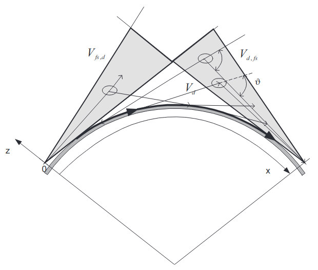
A combination of these four terms may provide observable levels of the scattered field as well as frequency and height dependence in agreement with experiment.

- Ivanov, V., Kinber, B., Korzenevitch, I. and Stepanov, B. Impact of the earth surface on long-range tropospheric propagation, Radiotech. Electron., 1980, 25 (10), 2033–2042.
- Saitchev, A., Slavinsky, M. Equations for moment-functions of waves propagating in random media with anisotropic inhomogeneities, Radiophys. Quant. Electron., 1985, 28 (1), 75–83.
- Kukushkin, A., Fuks, I. and Freilikher, V. Impact from random stratification on a coherent component of the field over horizon, Radiophys. Quant. Electron., 1983, 28 (8), 1064–1072.
- Long-range UHF Propagation in the Troposphere, Eds. Vvedensky, B., Kolosov, M., Kalinin, A. and Shifrin, J., Soviet Radio, Moscow, 1965, 416 pp.
- Shur, A. Signal Characteristics of Tropospheric Radiolinks, Swyaz, Moscow, 1972, 105 pp.
- Shifrin, J. Problems of Statistical Antenna Theory, Soviet Radio, Moscow, 1970, 384 pp.
- Kalinin, A., Troitzky, V. and Shur, A. The study of long-range UHF tropospheric propagation, in Radiowave Propagation , Eds. Kolosov, M., Armand, N., Katzelenbaum, B. and Sokolov, A., Nauka, Moscow, 1975, pp. 127– 153.
- Rytov, S.M., Kravtsov, Y.A. and Tatarskii, V.I. Introduction to Statistical Radiophysics: Part 2, Random Fields, Nauka, Moscow, 1978, 464 pp.
- Tatarskii, V.I. The Effects of Turbulent Atmosphere on Wave Propagation, IPST, Jerusalem, 1971.
- Feinberg, E. Radiowave Propagation over the Earth’s Surface, Nauka, Moscow, 1961, 547 pp.
- Booker, H., Gordon, W. A theory of radio scattering in the troposphere, 1950, Proc. IRE, 1950, 38 (4), 401–412.
- Klatskin, V.I. Stochastic Equations and Waves in Random Media, Nauka, Moscow, 1980, 336 pp.
- Rotheram, S. Radiowave propagation in the evaporation duct, 1974, The Marconi Rev., 1974, 37 (192), 18–40.