The efficient and safe movement of hydrocarbons is the cornerstone of the oil and gas industry. Within the complex network of wells, pipelines, and processing facilities, the dynamics of fluid transport are rarely simple. Instead of a single, uniform phase, engineers must contend with multiphase flow, which involves the simultaneous transport of oil, gas, and water.
Understanding and accurately predicting the behavior of these co-current phases is paramount for successful design and operation. This article serves as a comprehensive guide to the essential concepts and methodologies used in this critical engineering discipline.
- Introduction
- Multiphase Flow Terminology
- Superficial Velocity
- Multiphase Flow Mixture Velocity
- Holdup
- Phase Velocity
- Slip
- Multiphase Flow Density
- Multiphase Flow Regimes
- Two-Phase Flow Regimes
- Three-Phase Flow Regimes
- Calculating Multiphase Flow Pressure Gradients
- Steady-State Two-Phase Flow
- Steady-State Three-Phase Flow
- Transient Multiphase Flow
- Multiphase Flow in Gas/Condensate Pipelines
- Temperature Profile of Multiphase pipelines
- Three-phase Flash Calculation for Hydrocarbon Systems Containing Water
We begin by establishing the fundamentals – defining key terminology such as superficial velocity, holdup, and slip – before exploring the characteristic flow regimes that govern how different phase distributions affect fluid movement. Crucially, the focus then shifts to the quantitative analysis: the Oil and Gas Multiphase Flow Calculations. We will delve into steady-state and transient modeling techniques necessary for determining pressure gradients, predicting temperature profiles, and managing complex gas/condensate systems.
Mastering these calculations is vital for ensuring flow assurance, optimizing production rates, and designing infrastructure that is both cost-effective and resilient against operational challenges.
Introduction
Natural gas is often found in places where there is no local market, such as in the many offshore fields around the world. For natural gas to be available to the market, it must be gathered, processed, and transported. Quite often, collected natural gas (raw gas) must be transported over a substantial distance in pipelines of different sizes. These pipelines vary in length between hundreds of feet to hundreds of miles, across undulating terrain with varying temperature conditions. Liquid condensation in pipelines commonly occurs because of the multicomponent nature of the transmitted natural gas and its associated phase behavior to the inevitable temperature and pressure changes that occur along the pipeline. Condensation subjects the raw gas transmission pipeline to two-phase, gas/condensate, flow transport. Hence, a better understanding of the flow characteristics is needed for the proper design and operation of pipelines. The problem of optimal design of such pipelines becomes accentuated for offshore gas fields, where space is limited and processing often is kept to a minimum; therefore, total production has to be transported via multiphase pipelines.
These lines lie at the bottom of the ocean in horizontal and near-horizontal positions and may contain a three-phase mixture of hydrocarbon condensate, water (occurring naturally in the reservoir), and natural gas flowing through them.
Multiphase transportation technology has become increasingly important for developing marginal fields, where the trend is to economically transport unprocessed well fluids via existing infrastructures, maximizing the rate of return and minimizing both capital expenditure (CAPEX) and operational expenditure (OPEX). In fact, by transporting multiphase well fluid in a single pipeline, separate pipelines and receiving facilities for separate phases, costing both money and space, are eliminated, which reduces capital expenditure. However, phase separation and reinjection of water and gas save both capital expenditure and operating expenditure by reducing the size of the fluid transport/handling facilities and the maintenance required for the Pipelines in Marine Terminals: Key Considerations for Handling Liquefied Gaspipeline operation.
Given the savings that can be available to the operators using multiphase technology, the market for multiphase flow transportation is an expanding one. Hence, it is necessary to predict multiphase flow behavior and other design variables of gas-condensate pipelines as accurately as possible so that pipelines and downstream processing plants may be designed optimally. This chapter covers all the important concepts of multiphase gas/condensate transmission from a fundamental perspective.
Multiphase Flow Terminology
This section defines the variables commonly used to describe multiphase flow. For example, the general pressure drop equation for multiphase (two and three phase) flow is similar to that for single-phase flow except some of the variables are replaced with equivalent variables, which consider the effect of multiphase. The general pressure drop equation for multiphase flow is as follows:
where:
where:
- – is flow pressure gradient;
- x – is pipe length;
- ρ – is flow density;
- V – is flow velocity;
- f – is friction coefficient of flow;
- D – is internal diameter of pipeline;
- θ – is inclination angle of pipeline;
- g – is gravitational acceleration, and gc is gravitational constant.
The subscripts are “tot” for total, “ele” for elevation, “fri” for friction loss, “acc” for acceleration change terms, and “tp” for two- and/or three-phase flow.
Due to different flow mechanisms for different flow patterns, the multiphase (two/three phase) flow parameters used in the aforementioned pressure gradient equations should be defined separately. Definitions for commonly used multiphase variables are described based on Figure 1.
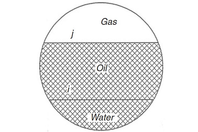
The ideal flow of three fluids is considered in Figure 1: water, oil, and gas. It is assumed that the water is heavier than the oil and flows at the bottom, while the oil flows in the middle and the gas is the top layer.
Superficial Velocity
The superficial velocity is the velocity of one phase of a multiphase flow, assuming that the phase occupies the whole cross section of pipe by itself.
It is defined for each phase as follows:
where:
The parameter A is the total cross-sectional area of pipe, Q is volumetric flow rate, V is velocity, and the subscripts are W for water, O for oil, G for gas, and S for superficial term.
Multiphase Flow Mixture Velocity
Mixture velocity is the sum of phase superficial velocities:
where:
- VM is the multiphase mixture velocity.
Holdup
Holdup is the cross-sectional area, which is locally occupied by one of the phases of a multiphase flow, relative to the cross-sectional area of the pipe at the same local position.
For the liquid phase,
For the gas phase,
where the parameter H is the phase holdup and the subscripts are L for the liquid and G for the gas phase.
Read also: Properties and hazards of shipping LNG, LPG
Although “holdup” can be defined as the fraction of the pipe volume occupied by a given phase, holdup is usually defined as the in situ liquid volume fraction, whereas the term “void fraction” is used for the in situ gas volume fraction.
Phase Velocity
Phase velocity (in situ velocity) is the velocity of a phase of a multiphase flow based on the area of the pipe occupied by that phase. It may also be defined for each phase as follows:
Slip
Slip is the term used to describe the flow condition that exists when the phases have different phase velocities. The slip velocity is defined as the difference between actual gas and liquid velocities, as follows:
The ratio between two-phase velocities is defined as the slip ratio. If there is no slip between the phases, VL = VG, and by applying the no-slip assumption to the liquid holup definition, it can be shown that
Investigators have observed that the no-slip assumption is not often applicable. For certain flow patterns in horizontal and upward inclined pipes, gas tends to flow faster than the liquid (positive slip). For some flow regimes in downward flow, liquid can flow faster than the gas (negative slip).
Multiphase Flow Density
Equations for two-phase gas/liquid density used by various investigators are as follows:
Equation 16 is used by most investigators to determine the pressure gradient due to elevation change. Some correlations are based on the assumption of no slippage and therefore use Equation 17 for two-phase density. Equation 18 is used by some investigators to define the density used in the friction loss term and in the Reynolds number. In the equations shown earlier, the total liquid density can be determined from the oil and water densities and flow rates if no slippage between these liquid phases is assumed:
where:
where the parameter f is the volume fraction of each phase.
Multiphase Flow Regimes
Multiphase flow is a complex phenomenon that is difficult to understand, predict, and model. Common single-phase flow characteristics such as velocity profile, turbulence, and boundary layer are thus inappropriate for describing the nature of such flows. The flow structures are rather classified in flow regimes, whose precise characteristics depend on a number of parameters. Flow regimes vary depending on operating conditions, fluid properties, flow rates, and the orientation and geometry of the pipe through which the fluids flow. The transition between different flow regimes may be a gradual process. Due to the highly nonlinear nature of the forces that rule the flow regime transitions, the prediction is near impossible.
It will be interesting: Personal protection of crew on Gas Carriers
In the laboratory, the flow regime may be studied by direct visual observation using a length of transparent piping. However, the most utilized approach is to identify the actual flow regime from signal analysis of sensors whose fluctuations are related to the flow regime structure. This approach is generally based on average cross-sectional quantities, such as pressure drop or cross-sectional liquid holdup. Many studies have been documented using different sensors and different analysis techniques.
In order to obtain optimal design parameters and operating conditions, it is necessary to clearly understand two- and three-phase flow regimes and the boundaries between them, where the hydrodynamics of the flow, as well as the flow mechanisms, change significantly from one flow regime to another. If an undesirable flow regime is not anticipated in the design, the resulting flow pattern can cause system pressure fluctuation and system vibration and even mechanical failures of Piping System of pressure vessels on gas tankerspiping components.
Two-Phase Flow Regimes
The description of two-phase flow can be simplified by classifying types of gas-liquid interfacial distribution and calling these “flow regimes” or “flow patterns“. The distribution of the fluid phases in space and time differs for the various flow regimes and is usually not under the control of the pipeline designer or operator.
Horizontal Flow Regimes
Two-phase flow regimes for horizontal flow are shown in Figure 2. These horizontal flow regimes are defined as follows.
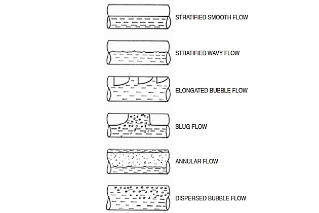
Stratified (Smooth and Wavy) Flow Stratified flow consists of two superposed layers of gas and liquid, formed by segregation under the influence of gravity. The gas-liquid interface is more or less curved and either smooth or rough because of capillary or gravity forces. The curvature of the interface increases with the velocity of the gas phase.
Intermittent (Slug and Elongated Bubble) Flow The intermittent flow regime is usually divided into two subregimes: plug or elongated bubble flow and slug flow. The elongated bubble flow regime can be considered as a limiting case of slug flow, where the liquid slug is free of entrained gas bubbles. Although these flow regimes are quite similar to each other, their fluid dynamic characteristics are very different and greatly influence such quantities as pressure drop and slug velocity. Gas-liquid intermittent flow exists in the whole range of pipe inclinations and over a wide range of gas and liquid flow rates. It is characterized by an intrinsic unsteadiness due to regions in which the liquid slugs fill the whole pipeline cross section and regions in which the flow consists of a liquid layer and a gas layer. The presence of these slugs can often be troublesome in the practical applications (giving rise to sudden pressure pulses, causing large system vibration and surges in liquid and gas flow rates), and the prediction of the onset of slug flow is of considerable industrial importance.
Annular Flow During annular flow, the liquid phase flows largely as an annular film on the wall with gas flowing as a central core. Some of the liquid is entrained as droplets in this gas core. The annular liquid film is thicker at the bottom than at the top of the pipe because of the effect of gravity and, except at very low liquid rates, the liquid film is covered with large waves.
Read also: Gas Tanker Equipment and Instrumentation
Dispersed Bubble Flow At high liquid rates and low gas rates, the gas is dispersed as bubbles in a continuous liquid phase. The bubble density is higher toward the top of the pipeline, but there are bubbles throughout the cross section. Dispersed flow occurs only at high flow rates and high pressures. This type of flow, which entails high-pressure loss, is rarely encountered in flow lines.
Note that raw gas pipelines usually have stratified smooth/wavy flow patterns. This arises because flow lines are designed to have appreciable velocities and the liquid content is usually quite low. Annular flow can also occur but this corresponds to high velocities, which are avoided to prevent erosion/corrosion, etc. In other words, raw gas lines are “sized” to be operated in stratified flow during normal operation.
Vertical Flow Regimes
Flow regimes frequently encountered in upward vertical two-phase flow are shown in Figure 3. These flow regimes tend to be somewhat more simpler than those in horizontal flow. This results from the symmetry in the flow induced by the gravitational force acting parallel to it. A brief description of the manner in which the fluids are distributed in the pipe for upward vertical two-phase flow is as follows. It is worth noting that vertical flows are not so common in raw gas systems (i. e., wells normally have some deviation and many risers are also inclined to some extent).
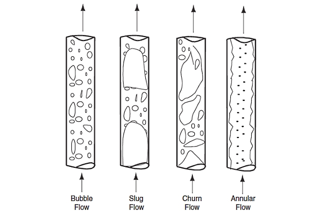
Bubble Flow The gas phase is distributed in the liquid phase as variable-size, deformable bubbles moving upward with zigzag motion. The wall of the pipe is always contacted by the liquid phase.
Slug Flow Most of the gas is in the form of large bullet-shaped bubbles that have a diameter almost reaching the pipe diameter. These bubbles are referred to as “Taylor bubbles“, move uniformly upward, and are separated by slugs of continuous liquid that bridge the pipe and contain small gas bubbles. Typically, the liquid in the film around the Taylor bubbles may move downward at low velocities, although the net flow of liquid can be upward. The gas bubble velocity is greater than that of the liquid.
Churn Flow If a change from a continuous liquid phase to a continuous gas phase occurs, the continuity of the liquid in the slug between successive Taylor bubbles is destroyed repeatedly by a high local gas concentration in the slug. This oscillatory flow of the liquid is typical of churn flow. It may not occur in small-diameter pipes. The gas bubbles may join and liquid may be entrained in the bubbles.
Annular Flow Annular flow is characterized by the continuity of the gas phase in the pipe core. The liquid phase moves upward partly as a wavy film and partly in the form of drops entrained in the gas core. Although downward vertical two-phase flow is less common than upward flow, it does occur in steam injection wells and down comer pipes from offshore production platforms. Hence a general vertical two-phase flow pattern is required that can be applied to all flow situations. Reliable models for downward multiphase flow are currently unavailable and the design codes are deficient in this area.
Inclined Flow Regimes
The effect of pipeline inclination on the gas-liquid two-phase flow regimes is of a major interest in hilly terrain pipelines that consist almost entirely of uphill and downhill inclined sections. Pipe inclination angles have a very strong influence on flow pattern transitions. Generally, the flow regime in a near-horizontal pipe remains segregated for downward inclinations and changes to an intermittent flow regime for upward inclinations. An intermittent flow regime remains intermittent when tilted upward and tends to segregated flow pattern when inclined downward. The inclination should not significantly affect the distributed flow regime.
Flow Pattern Maps
The boundaries of different gas-liquid two-phase flow regimes have been determined experimentally and reported in the literature. The results of experimental studies are generally presented as a flow pattern map. The respective pattern may be represented as areas on a plot, the coordinates of which are the dimensional variables (i. e., superficial phase velocities) or dimensionless parameters containing these velocities. Although plots are useful in representing data, they are limited to the particular sets of conditions investigated and there is an obvious need to generalize flow pattern information so that it can be applied to any pair of fluids and any geometry. A more flexible method, which overcomes this difficulty, is to examine each transition individually and derive a criterion valid for that particular transition.
It will be interesting: Basic Info about Liquefied Petroleum Gas Transportation on the LPG tankers
For horizontal flows, the classical map is that of Baker, which is widely used in the petroleum industry. The original Baker diagram is shown in Figure 4. The map is based on air-water data at atmospheric pressure in 1-, 2-, and 4-inch pipes.
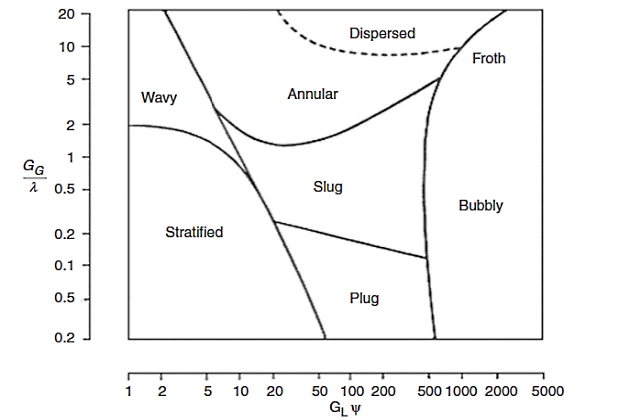
The abscissa is the superficial mass velocity of the liquid phase (GL) and the ordinate is the superficial mass velocity of the gas phase (GG) and both coordinates have been corrected for physical properties of the respective phases. These parameters are given by the following relationships:
where:
- m – is mass flow rate, lbm/hr;
- A – is pipe cross section, ft2;
- σ – is surface tension, dynes/ft;
- and µ is viscosity, lb/ft.s.
The subscripts A and W refer to the values of the physical properties for air and water, respectively, at atmospheric pressure and temperature.
For vertical gas-liquid two-phase flow, the flow pattern map of Hewitt and Roberts is shown in Figure 5.
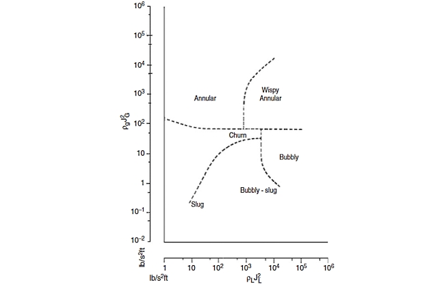
Fig. 5 Flow pattern map for vertical flow (Hewitt and Roberts, 1969)
This map has been obtained from observations on low-pressure air-water and high-pressure steam-water flow in small diameter (0,4-1,2 inch) vertical tubes.
Note that a word of warning should be issued about the use of flow pattern maps. For example, the use of superficial phase velocities for the axes of the map restricts its application to one particular situation. Therefore, they should be used with discretion serving as a general guide to the likely pattern rather than a positive indication that the pattern actually exists for a given situation. There have been some attempts to evaluate the basic mechanisms of flow pattern transitions and thus to provide a mechanistic flow pattern map for estimating their occurrence. In these transition models, the effects of system parameters are incorporated; hence they can be applied over a range of conditions.
However, most of them are somewhat complex and require the use of a predetermined sequence to determine the dominant flow pattern.
Three-Phase Flow Regimes
The main difference between two-phase (gas/liquid) flows and three-phase (gas/liquid/liquid) flows is the behavior of the liquid phases, where in three-phase systems the presence of two liquids gives rise to a rich variety of flow patterns. Basically, depending on the local conditions, the liquid phases appear in a separated or dispersed form. In the case of separated flow, distinct layers of oil and water can be discerned, although there may be some interentrainment of one liquid phase into the other. In dispersed flow, one liquid phase is completely dispersed as droplets in the other, resulting in two possible situations, namely an oil continuous phase and a water continuous phase. The transition from one liquid continuous phase to the other is known as phase inversion. If the liquid phases are interdispersed, then prediction of phase inversion is an important item. For this purpose, Decarre and Fabre developed a phase inversion model that can be used to determine which of two liquids is continuous.
Due to the many possible transport properties of three-phase fluid mixtures, the quantification of three-phase flow pattern boundaries is a difficult and challenging task. Acikgoz et al. observed a very complex array of flow patterns and described 10 different flow regimes. In their work, the pipe diameter was only 0,748 inch and stratification was seldom achieved. In contrast, the Lee et al. experiments were carried out in a 4-inch-diameter pipe. They observed and classified seven flow patterns, which were similar to those of two-phase flows:
- smooth strat-ified,
- wavy stratified,
- rolling wave,
- plug flow,
- slug flow,
- pseudo slug,
- and annular flow.
The first three flow patterns can be classified as stratified flow regime and they noted that the oil and the water are generally segregated, with water flowing as a liquid layer at the bottom of the pipe and oil flowing on top. Even for plug flow, the water remained at the bottom because agitation of the liquids was not sufficient to mix the oil and water phases. Note that turbulence, which naturally exists in a pipeline, can be sufficient to provide adequate mixing of the water and oil phase. However, the minimum natural turbulent energy for adequate mixing depends on the oil and water flow rates, pipe diameter and inclination, water concentration, viscosity, density, and interfacial tension. Dahl et al. provided more detailed information on the prediction methods that can be used to determine whether a water-in-oil mixture in the pipe is homogeneous or not.
Calculating Multiphase Flow Pressure Gradients
The hydraulic design of a multiphase flow pipeline is a two-step process. The first step is the determination of the multiphase flow regimes because many pressure drop calculation methods rely on the type of flow regime present in the pipe. The second step is the calculation of flow parameters, such as pressure drop and liquid holdup, to size pipelines and field processing equipment, such as slug catchers.
Steady-State Two-Phase Flow
The techniques used most commonly in the design of a two-phase flow pipeline can be classified into three categories:
- single-phase flow approaches;
- homogeneous flow approaches;
- and mechanistic models.
Within each of these groups are subcategories that are based on the general characteristics of the models used to perform design calculations.
Single-Phase Flow Approaches
In this method, the two-phase flow is assumed to be a single-phase flow having pseudo-properties arrived at by suitably weighting the properties of the individual phases. These approaches basically rely solely on the well-established design equations for single-phase gas flow in pipes. Two-phase flow is treated as a simple extension by use of a multiplier: a safety factor to account for the higher pressure drop generally encountered in two-phase flow. This heuristic approach was widely used and generally resulted in inaccurate pipeline design.
Read also: Gas Tank Environmental Control
In the past, single-phase flow approaches were used commonly for the design of wet gas pipelines. When the amount of the condensed liquid is negligibly small, the use of such methods could at best prevent underdesign, but more often than not, the quantity of the condensed liquid is significant enough that the single-phase flow approach grossly overpredicted the pressure drop. Hence, this method is not covered in depth here but can be reviewed elsewhere.
Homogeneous Flow Approaches
The inadequacy of the single-phase flow approaches spurred researchers to develop better design procedures and predictive models for two-phase flow systems. This effort led to the development of homogeneous flow approaches to describe these rather complex flows. The homogeneous approach, also known as the friction factor model, is similar to that of the single-phase flow approach except that mixture fluid properties are used in determination of the friction factor. Therefore, the appropriate definitions of the fluid properties are critical to the accuracy of the model. The mixture properties are expressed empirically as a function of the gas and liquid properties, as well as their respective holdups.
Many of these correlations are based on flow regime correlations that determine the two-phase (gas/liquid) flow friction factor, which is then used to estimate pressure drop. While some of the correlations predict pressure drop reasonably well, their range of applicability is generally limited, making their use as a scale up tool marginal. This limitation is understandable because the database used in developing these correlations is usually limited and based on laboratory-scale experiments.
Extrapolation of these data sets to larger lines and hydrocarbon systems is questionable at best. Blind application of these correlations can lead to results, which are marginal, resulting in two-phase equipment overdesign leading to unnecessary costs or even failure. However, many of these correlations have been used for lack of other design means and two of which are outlined in the following section. In-depth comparative analyses of the available homogeneous flow approaches have been reported by Brill and Beggs and Collier and Thome.
Lockhart and Martinelli Method This method was developed by correlating experimental data generated in horizontal isothermal two-phase flow of two-component systems (air-oil and air-water) at low pressures (close to atmospheric) in a 1-inch-diameter pipe. Lockhart and Martinelli separated data into four sets dependent on whether the phases flowed in laminar or turbulent flow, if the phases were flowing alone in the same pipe. In this method, a definite portion of the flow area is assigned to each phase and it is assumed that the single-phase pressure drop equations can be used independently for each phase. The two-phase frictional pressure drop is calculated by multiplying by a correction factor for each phase, as follows:
where:
The friction factors fG and fL are determined from the Moody diagram using the following values of the Reynolds number:
The two-phase flow correction factors (ϕG, ϕL) are determined from the relationships of Equations 30 and 31:
where
where parameter C has the values shown in Table 1. Note that the laminar flow regime for a phase occurs when the Reynolds number for that phase is less than 1 000.
| Table 1. “C” Parameter | ||
|---|---|---|
| Liquid phase | Gas phase | C |
| Turbulent | Turbulent | 20 |
| Laminar | Turbulent | 12 |
| Turbulent | Laminar | 10 |
| Laminar | Laminar | 5 |
In this method, the correlation between liquid holdup and Martinelli parameter, X, is independent of the flow regime and can be expressed as follows:
The fluid acceleration pressure drop was ignored in this method. However, the extension of the work covering the estimation of the accelerative term was done by Martinelli and Nelson. Although different modifications of this method have been proposed, the original method is believed to be generally the most reliable.
Beggs and Brill Method This method was developed from 584 experimental data sets generated on a laboratory-scale test facility using an air-water system. The facility consisted of 90 feet of 1- or 1,5-inch-diameter acrylic (smooth) pipe, which could be inclined at any angle. The pipe angle was varied between horizontal to vertical and the liquid holdup and the pressure were measured. For each pipe size in the horizontal position, flow rates of two phases were varied to achieve all flow regimes. Beggs and Brill developed correlations for the liquid holdup for each of three horizontal flow regimes and then corrected these for the pipe inclination/angle.
The following parameters are used for determination of all horizontal flow regimes:
The flow regimes limits are:
Segregated
Transition
Intermittent
Distributed
Also, the horizontal liquid holdup, HL(0), is calculated using the following equation:
where parameters a, b, and c are determined for each flow regime and are given in Table 2. With the constraint that HL(0) ≥ λL.
| Table 2. a, b, c Parameters | |||
|---|---|---|---|
| Flow regime | a | b | c |
| Segregated | 0,98 | 0,4846 | 0,0868 |
| Intermittent | 0,845 | 0,5351 | 0,0173 |
| Distributed | 1,065 | 0,5824 | 0,0609 |
When the flow is in the transition region, the liquid holdup is calculated by interpolating between the segregated and the intermittent flow regimes as follows:
where:
The amount of liquid holdup in an inclined pipe, HL(θ), is determined by multiplying an inclination factor (Ψ) by the calculated liquid holdup for the horizontal conditions:
where:
where θ is the pipe angle and α is calculated as follows:
where:
The equation parameters are determined from each flow regime using the numbers from Table 3.
| Table 3. d, e, f, and g Parameters | ||||
|---|---|---|---|---|
| Flow regime | d | e | f | g |
| Segregated uphill | 0,011 | -3,768 | 3,539 | -1,614 |
| Intermittent uphill | 2,96 | 0,305 | -0,4473 | 0,0978 |
| Distributed uphill | ||||
| All flow regimes downhill | 4,7 | -0,3692 | 0,1244 | -0,5056 |
The two-phase pressure gradient due to pipeline elevation can be determined as follows:
Also, the two-phase frictional pressure drop is calculated as:
where:
where fn is the no-slip friction factor determined from the smooth pipe curve of the Moody diagram using no-slip viscosity and the density in calculating the two-phase flow Reynolds number. In other words,
where:
The exponent β is given by
where:
The pressure drop due to acceleration is only significant in gas transmission pipelines at high gas flow rates. However, it can be included for completeness as:
The Beggs and Brill method can be used for horizontal and vertical pipelines, although its wide acceptance is mainly due to its usefulness for inclined pipe pressure drop calculation. However, the proposed approach has limited applications dictated by the database on which the correlations are derived.
Note that the Beggs and Brill correlation is not usually employed for the design of wet gas pipelines. Specifically the holdup characteristic (holdup versus flow rate) is not well predicted by this method. This makes design difficult because one is unable to reliably quantify the retention of liquid in the line during turndown conditions.
Mechanistic Models
While it is indeed remarkable that some of the present correlations can adequately handle noncondensing two-phase flow, they give erroneous results for gas-condensate flow in large-diameter lines at high pressures. This shortcoming of existing methods has led to the development of mechanistic models based on fundamental laws and thus can offer more accurate modeling of the pipe geometric and fluid property variations. All of these models predict a stable flow pattern under the specified conditions and then use momentum balance equations to calculate liquid holdup, pressure drop, and other two-phase flow parameters with a greater degree of confidence than that possible by purely empirical correlations.
Read also: Piping System of pressure vessels on gas tankers
The mechanistic models presented in the literature are either incomplete in that they only consider flow pattern determination or are limited in their applicability to only some pipe inclinations or small-diameter, low-pressure two-phase flow lines. However, new mechanistic models presented by Petalas and Aziz and Zhang et al. have proven to be more robust than previous models, although further investigations and testing of these models are needed with high-quality field and laboratory data in larger diameter, high-pressure systems. Readers are referred to the original references for a detailed treatment of these models.
Steady-State Three-Phase Flow
Compared to numerous investigations of two-phase flow in the literature, there are only limited works on three-phase flow of gas-liquid-liquid mixtures. In fact, the complex nature of such flows makes prediction very difficult. In an early study, Tek treated the two immiscible liquid phases as a single fluid with mixture properties, thus a two-phase flow correlation could be used for pressure loss calculations. Studies by Pan have shown that the classical two-phase flow correlations for gas-liquid two-phase flow can be used as the basis in the determination of three-phase flow parameters; however, the generality of such empirical approaches is obviously questionable. Hence, an appropriate model is required to describe the flow of one gas and two liquid phases.
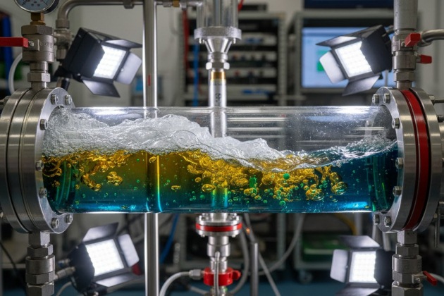
Source: AI generated image
One of the most fundamental approaches used to model such systems is the two-fluid model, where the presented approach can be used by combining the two liquid phases as one pseudo-liquid phase and modeling the three-phase flow as a two-phase flow. However, for more accurate results, three-fluid models should be used to account for the effect of liquid-liquid interactions on flow characteristics, especially at low flow rates. Several three fluid models were found in the literature. All of these models are developed from the three-phase momentum equations with few changes from one model to the other. The most obvious model has been developed by Barnea and Taitel; however, such a model introduces much additional complexity and demands much more in computer resources compared with the two-fluid model for two-phase flow.
Transient Multiphase Flow
Transient multiphase flow in pipelines can occur due to changes in inlet flow rates, outlet pressure, opening or closing of valves, blowdown, ramp-up, and pigging. In each of these cases, detailed information of the flow behavior is necessary for the designer and the operator of the system to construct and operate the pipeline economically and safely.
The steady-state pipeline design tools are not sufficient to adequately design and confirm the operational flexibility of multiphase pipelines. Therefore, a model for predicting the overall flow behavior in terms of pressure, liquid holdup, and flow rate distributions for these different transient conditions would be very useful. Some current research challenges in modeling transient flow relate to an understanding and formulation of basic flow models for oil-water-gas flow and to numerical methods applicable for the solution of transient multiphase flows. These methods are available to some extent in multiphase fluid dynamics simulation codes, which are the key design tools for multiphase flow pipeline calculations.
Transient multiphase flow is traditionally modeled by one-dimensional averaged conservation laws, yielding a set of partial differential equations. In this section, two models of particular industrial interest are described.
- The two-fluid model (TFM), consisting of a separate momentum equation for each phase.
- The drift-flux model (DFM), consisting of a momentum equation and an algebraic slip relation for the phase velocities.
The TFM is structurally simpler, but involves an extra differential equation when compared to the DFM. They do yield somewhat different transient results, although the differences are often small.
The following major assumptions have been made in the formulation of the differential equations.
- Two immiscible liquid phases (oil and water) that are assumed to be a single fluid with mixture properties.
- Flow is one dimensional in the axial direction of the pipeline.
- Flow temperature is constant at wall, and no mass transfer occurs between gas and liquid phases. Note that most commercial codes allow phase change.
- The physical properties of multiphase flow are determined at the average temperature and pressure of flow in each segment of the pipeline.
Two-Fluid Model
The TFM is governed by a set of four partial differential equations, the first two of which express mass conservation for gas and liquid phases, respectively,
The last two equations represent momentum balance for the gas and liquid phases, respectively,
In Equations 55 and 56, parameter P denotes the interface pressure, whereas Vk, ρk, and Hk are the velocity, the density, and the volume fraction of phase k ∈ {G, L}, respectively. The variables τi and τk are the interfacial and wall momentum transfer terms. The quantities ∆PG and ∆PL correspond to the static head around the interface, defined as follows:
where:
- ω – is the wetted angle.
The detailed description of the solution algorithm for these equations is based on a finite volume method.
One major limitation of this type of model is the treatment of the interfacial coupling. While this is relatively easy for separated flows (stratified and annular), this treatment is intrinsically flawed for intermittent flows. Another drawback is that propagation phenomena, especially pressure waves, tend not to account for satisfactorily.
Drift Flux Model
The DFM is derived from the two-fluid model by neglecting the static head terms ∆PG and ∆PL in Equations 57 and 57 and replacing the two momentum equations by their sum. The main advantages of this three-equation model are as follows.
- The equations are in conservative form, which makes their solution by finite volume methods less onerous.
- The interfacial shear term, τi, is cancelled out in the momentum equations, although it appears in an additional algebraic relation called the slip law.
- The model is well posed and does not exhibit a complex characteristic.
Adding Equations 55 and 56 together yields:
The interfacial exchange term, τi, is no longer present in the aforementioned equation. This leads in the DFM to a new model that consists of three partial differential equations, i. e., Equations 53, 54, and 59. Additional model numerical solution details can be found in Faille and Heintze.
Note that the drift flux approach is best applied to closely coupled flows such as bubbly flow. Its application to stratified flows is, at best, artificial.
Multiphase Flow in Gas/Condensate Pipelines
Gas/condensate flow is a multiphase flow phenomenon commonly encountered in raw gas transportation. However, the multiphase flow that takes place in gascondensate transmission lines differs in certain respects from the general multiphase flow in pipelines. In fact, in gas/condensate flow systems, there is always interphase mass transfer from the gas phase to the liquid phase because of the temperature and pressure variations, which leads to compositional changes and associated fluid property changes. In addition, the amount of liquid in such systems is assumed to be small, and the gas flow rate gives a sufficiently high Reynolds number that the fluid flow regime for a nearly horizontal pipe can be expected to be annular-mist flow and/or stratified flow. For other inclined cases, even with small quantities of liquids, slug-type regimes may be developed if liquids start accumulating at the pipe lower section.
In order to achieve optimal design of gas/condensate pipelines and downstream processing facilities, one needs a description of the relative amount of condensate and the flow regime taking place along the pipelines, where fluid flowing in pipelines may traverse the fluid phase envelope such that the fluid phase changes from single phase to two phase or vice versa. Hence, compositional singlephase/multiphase hydrodynamic modeling, which couples the hydrodynamic model with the natural gas-phase behavior model, is necessary to predict fluid dynamic behavior in gas/condensate transmission lines. The hydrodynamic model is required to obtain flow parameters along the pipeline, and the phase behavior model is required for determining the phase condition at any point in the pipe, the mass transfer between the flowing phases, and the fluid properties.
Despite the importance of gas flow with low liquid loading for the operation of gas pipelines, few attempts have been made to study flow parameters in gas/condensate transmission lines. While the single-phase flow approaches have been applied previously to gas/condensate systems, only a few attempts have been reported for the use of the two-fluid model for this purpose. Some of them have attempted to make basic assumptions (e. g., no mass transfer between gas and liquid phases) in their formulation and others simply assume one flow regime for the entire pipe length. However, a compositional hydrodynamic model that describes the steady-state behavior of multiphase flow in gas/condensate pipelines has been presented by Ayala and Adewumi. The model couples a phase beh avior model, based on the Peng and Robinson equation of state, and a hydrodynamic model, based on the two-fluid model. The proposed model is a numerical approach, which can be used as an appropriate tool for engineering design of multiphase pipelines transporting gas and condensate.
It will be interesting: Overview of Alternative Propulsion Systems for the LNG Vessel
However, the complexity of this model precludes further discussion here. Note that the presence of liquid (condensates), in addition to reducing deliverability, creates several operational problems in gas-condensate transmission lines. Periodic removal of the liquid from the pipeline is thus desirable. To remove liquid accumulation in the lower portions of pipeline, pigging operations are performed. These operations keep the pipeline free of liquid, reducing the overall pressure drop increasing pipeline flow efficiency. However, the pigging process associates with transient flow behavior in the pipeline. Thus, it is imperative to have a means of predicting transient behavior encountered in multiphase, gas/gas-condensate pipelines. Until recently, most available commercial codes were based on the two-fluid model; however, the model needs many modifications to be suitable for simulating multiphase transient flow in gas/gas-condensate transmission lines. For example, the liquid and gas continuity equations need to be modified to account for the mass transfer between phases.
So far, several codes have been reported for this purpose, where three main commercial transient codes are OLGA, PROFES, and TACITE. Detailed discussion of these codes is beyond the scope of this book; readers are referred to the original papers for further information.
Temperature Profile of Multiphase pipelines
Predicting the flow temperature and pressure changes has become increasingly important for use in both the design and the operation of flow transmission pipelines. It is therefore imperative to develop appropriate methods capable of predicting these parameters for multiphase pipelines. A simplified flowchart of a suitable computing algorithm is shown in Figure 6. This algorithm calculates pressure and temperature along the pipeline by iteratively converging on pressure and temperature for each sequential “segment” of the pipeline.
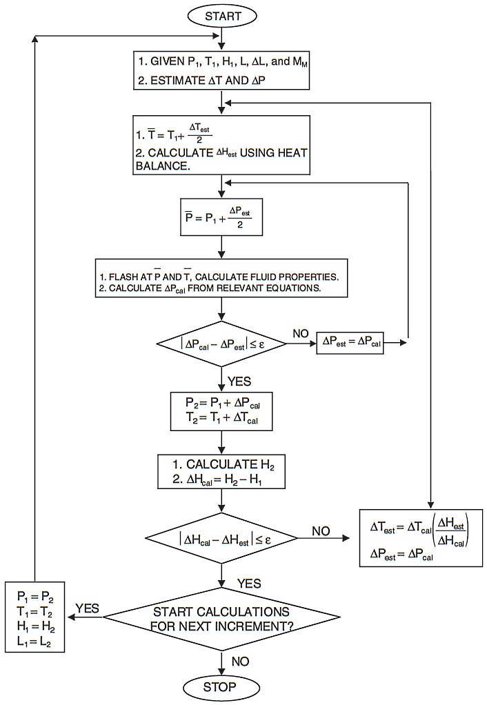
The algorithm converges on temperature in the outer loop and pressure in the inner loop because robustness and computational speed are obtained when converging on the least sensitive variable first.
The pipeline segment length should be chosen such that the fluid properties do not change significantly in the segment. More segments are recommended for accurate calculations for a system where fluid properties can change drastically over short distances. Often, best results are obtained when separate segments (with the maximum segment length less than about 10 % of total line length) are used for up, down, and horizontal segments of the pipeline.
Prediction of the pipeline temperature profile can be accomplished by coupling the pressure gradient and enthalpy gradient equations as follows.
where:
- ∆H – is enthalpy change in the calculation segment, Btu/lbm;
- VM – is velocity of the fluid, ft/sec;
- VSG – is superficial gas velocity, ft/sec;
- ∆P – is estimated change in pressure, psi;
- – is average pressure in calculation segment, psia;
- ∆Z – is change in elevation, ft;
- U – is overall heat transfer coefficient, Btu/hr-ft2-°F;
- D – is reference diameter on which U is based, ft;
- T – is estimated average temperature in calculation segment, °F;
- Ta – is ambient temperature, °F;
- ∆L – is change in segment length, ft;
- and MM – is gas-liquid mixture mass flow rate, lbm/s.
As can be seen from Equation 60, temperature and pressure are mutually dependent variables so that generating a very precise temperature profile requires numerous iterative calculations. The temperature and pressure of each pipe segment are calculated using a double-nested procedure in which for every downstream pressure iteration, convergence is obtained for the downstream temperature by property values evaluated at the average temperature and pressure of that section of pipe. Experience shows that it is essential to use a good pressure-drop model to assess the predominant parameter, i. e., pressure.
The overall heat transfer coefficient (U) can be determined by a combination of several coefficients, which depend on the method of heat transfer and pipe configuration. Figure 7 is a cross section of a pipe, including each “layer” through which heat must pass to be transferred from the fluid to the surroundings or vice versa. This series of layers has an overall resistance to heat transfer made up of the resistance of each layer.
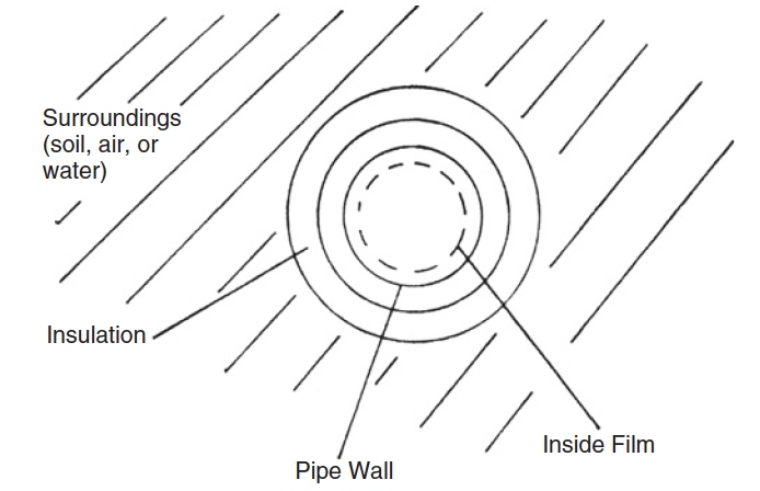
Fig. 7 Cross section of a pipe showing resistance layers
In general, the overall heat transfer coefficient for a pipeline is the reciprocal of the sums of the individual resistances to heat transfer, where each resistance definition is given in Table 4.
| Table 4. Types of Resistance Layers for a Pipe | |
|---|---|
| Resistance | Due to |
| Rinside, film | Boundary layer on the inside of the pipe |
| Rpipe | Material from which the pipe is made |
| Rinsulation | Insulation (up to five concentric layers) |
| Rsurr | Surroundings (soil, air, water) |
The individual resistances are calculated from the given equations in Table “Velocity Criteria for Sizing Multiphase PipelinesHeat Transfer Resistances for Pipes“.
Since fluid properties are key inputs into calculations such as pressure drop and heat transfer, the overall simulation accuracy depends on accurate property predictions of the flowing phases. Most of the required physical and thermodynamic properties of the fluids are derived from the equation of state. However, empirical correlations are used for the calculation of viscosity and surface tension. When the physical properties of the fluids are calculated for two-phase flow, the physical properties of the gas and liquid mixture can be calculated by taking the mole fraction of these components into account. Similarly, when water is present in the system, the properties of oil and water are combined into those of a pseudo-liquid phase. To produce the phase split for a given composition, pressure, and temperature, an equilibrium flash calculation utilizing an appropriate equation of state must be used. A simple and stable three-phase flash calculation with significant accuracy for pipeline calculation has been described by Mokhatab (see “Three-phase Flash Calculation for Hydrocarbon Systems Containing Water” below).
Three-phase Flash Calculation for Hydrocarbon Systems Containing Water
One of the most important engineering problems encountered in modeling chemical and petroleum processes is the multiphase flash problem. The present flash algorithm can be used to calculate phase equilibria for multicomponent systems with three coexisting phases (water, oil, and gas) at equilibrium with both simplicity and accuracy.
This three-hase flash algorithm is based on the thermodynamic condition of equal fugacities for each component in each phase. The resulting phase compositions then provide better values for updating the distribution coefficients using an equation of state (EOS). Equations of state have been used successfully to describe the phase behavior of reservoir crude and gas condensates, but the phase behavior of water/reservoir crude oil has not yet been predicted successfully by an EOS. In this study, it is demonstrated that using the present algorithm with the Shinta and Firoozabadi association model provides reliable and better results in comparison with experimental data for three-phase flash calculation in the vapor-liquid-liquid region.
A generalized model of a three-phase equilibrium system is shown in Figure 8. The phases are assumed to be in thermodynamic equilibrium with each other and any component can appear in all three phases.
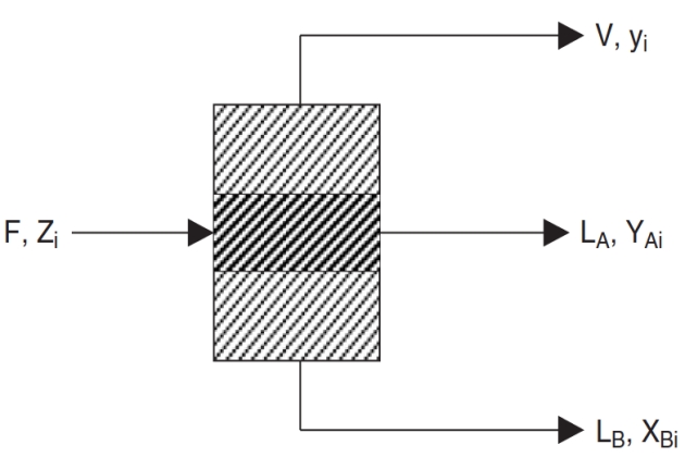
The overall and component material balance around the flash tank gives
where:
- F – is total moles of feed, lbmole;
- LA – is total moles of hydrocarbon-rich liquid, lbmole;
- LB – is total moles of water-rich liquid, lbmole;
- V – is total moles of vapor, lbmole;
- Zi – is mole fraction of component i in the feed;
- XAi – is mole fraction of component i in the hydrocarbon-rich liquid phase;
- XBi – is mole fraction of component i in the water-rich liquid phase;
- yi – is mole fraction of component i in the vapor phase.
The relations describing compositions in each phase that must be satisfied are:
where:
- i – is indicates each component;
- and n is the number of components.
Also the equilibrium relations between the compositions of each phase are defined by the following expressions:
where:
- KAi – is equilibrium ratio of component i in the hydrocarbon-rich liquid phase;
- KBi – is equilibrium ratio of component i in the water-rich liquid phase;
- – is fugacity coefficient of component i in the hydrocarbon-rich liquid phase;
- – is fugacity coefficient of component i in the water-rich liquid phase.
Combining Equations 61 through 65 gives the following equations:
The combining of the these equations can then be used to determine the phase and volumetric properties of the three-phase systems.
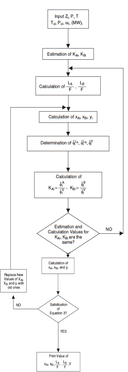
Peng and Robinson proposed the following equations for three-phase flash calculations:
Provided that the equilibrium ratios and the overall composition are known, the aforementioned equations can be solved simultaneously by using the modified Rachford and Rice iterative method. In the course of making phase equilibrium calculations, it is always desirable to provide initial values for the equilibrium ratios so the iterative procedure can proceed as reliably and rapidly as possible. Peng and Robinson adopted Wilson’s equilibrium ratio correlation to provide initial KA values, as follow:
where:
- P – is system pressure, psia;
- T – is system temperature, °F;
- PCi – is critical pressure of component i, psia;
- TCi – is critical temperature of component i, °F;
- and ωi – is acentric factor of component i.
While for determination of initial KB values, Peng and Robison proposed the following expression:
A logic diagram for three-phase flash calculations is shown in Figure 9.
In this method, the fugacity coefficients can be obtained from Peng and Robinson EOS for nonpolar compounds. Note that in the association equation of state, the compressibility factor of the association component such as water is subdivied into two physical and chemical parts as follow:
The physical compressibility factor, Zph, can be obtained from modified Peng and Robinson EOS. To evalute Zch in Equation 72, the Shinta and Firoozabadi association model is used. Also, the fugacity coefficient of an associating component in each phase is the sum of both chemical and physical contributions as follows:
where chemical fugacity coefficients are obtained by the Shinta and Firoozabadi association model. Note that in using the AEOS, only binary interaction coefficients between water and hydrocarbon, and nonhydrocarbon components and hydrocarbon cuts are required because calculations are often very sensitive to those. Therefore, in this method, binary interaction coefficients suggested by Nishiumi and Arai, Peng and Robinson, and Shinta and Firoozabadi are used.

- Acikgoz, M., Franca, F., and Lahey Jr, R. T., An experimental study of three-phase flow regimes. Int. J. Multiphase Flow 18(3), 327–336 (1992).
- Adewmi, M. A., and Bukacek, R. F., Two-phase pressure drop in horizontal pipelines. J. Pipelines 5, 1–14 (1985).
- Amdal, J., et al., “Handbook of Multiphase Metering.” Produced for The Norwegian Society for Oil and Gas Measurement, Norway (2001).
- Ansari, A. M., Sylvester, A. D., Sarica, C., Shoham, O., and Brill, J. P., A comprehensive mechanistic model for upward two-phase flow in wellbores. SPE Prod. Facilit. J. 143–152 (May 1994).
- API, “Computational Pipeline Monitoring.” API Publication 1130, 17, American Petroleum Institute, TX (1995a).
- API, “Evaluation Methodology for Software Based Leak Detection Systems.” API Publication 1155, 93, American Petroleum Institute, TX (1995b).
- API RP 14E, “Recommended Practice for Design and Installation of Offshore Production Platform Piping Systems,” 5th Ed., p. 23.
- Asante, B., “Two-Phase Flow: Accounting for the Presence of Liquids in Gas Pipeline Simulation.” Paper presented at 34th PSIG Annual Meeting, Portland, Oregon (Oct. 23–25, 2002).
- AsphWax’s Flow Assurance course, “Fluid Characterization for Flow Assurance.” AsphWax Inc., Stafford, TX (2003).
- Ayala, F.L., and Adewumi, M. A., Low-liquid loading multiphase flow in natural gas pipelines. ASME J. of Energy Res. Technol. 125, 284–293 (2003).
- Baillie, C., and Wichert, E., Chart gives hydrate formation temperature for natural gas. Oil Gas J. 85(4), 37–39 (1987).
- Baker, O., Design of pipelines for simultaneous flow of oil and gas. Oil Gas J. 53, 185 (1954).
- Banerjee, S., “Basic Equations.” Lecture presented at the Short Course on Modeling of Two-Phase Flow Systems, ETH Zurich, Switzerland (March 17–21, 1986).
- Barnea, D., A unified model for prediction flow pattern transitions for the whole range of pipe inclinations. Int. J. Multiphase Flow 13(1), 1–12 (1987).
- Barnea, D., and Taitel, Y., Stratified three-phase flow in pipes: Stability and transition. Chem. Eng. Comm. 141–142, 443–460 (1996).
- Battara, V., Gentilini, M., and Giacchetta, G., Condensate-line correlations for calculating holdup, friction compared to field data. Oil Gas J. 30, 148–52 (1985).
- Bay, Y., “Pipelines and Risers,” Vol. 5. Elsevier Ocean Engineering Book Series (2001).
- Beggs, H.D., and Brill, J. P., “A Study of Two-Phase Flow in Inclined Pipes.” JPT, 607–17; Trans., AIME, 255 (May 1973).
- Bendiksen, K., Brandt, I., Jacobsen, K. A., and Pauchon, C., “Dynamic Simulation of Multiphase Transportation Systems.” Multiphase Technology and Consequence for Field Development Forum, Stavanger, Norway (1987).
- Bendiksen, K., Malnes, D., Moe, R., and Nuland, S., The dynamic two-fluid model OLGA: Theory and application. SPE Prod. Eng. 6, 171–180 (1991).
- Bertola, V., and Cafaro, E., “Statistical Characterization of Subregimes in Horizontal Intermittent Gas/Liquid Flow.” Proc. the 4th International Conference on Multiphase Flow, New Orleans, LA (2001).
- Bjune, B., Moe, H., and Dalsmo, M., Upstream control and optimization increases return on investment. World Oil 223, 9 (2002).
- Black, P. S., Daniels, L. C., Hoyle, N. C., and Jepson, W. P., Studying transient multiphase flow using the pipeline analysis code (PLAC). ASME J. Energy Res. Technol. 112, 25–29 (1990).
- Bloys, B., Lacey, C., and Lynch, P., “Laboratory Testing and Field Trial of a New Kinetic Hydrate Inhibitor.” Proc. 27th Annual Offshore Technology Conference, OTC 7772, PP. 691–700, Houston, TX (1995).
- Bonizzi, M., and Issa, R. I., On the simulation of three-phase slug flow in nearly horizontal pipes using the multi-fluid model. Int. J. Multiphase Flow 29, 1719–1747 (2003).
- Boriyantoro, N. H., and Adewumi, M. A., “An Integrated Single-Phase/Two-Phase Flow Hydrodynamic Model for Predicting the Fluid Flow Behavior of Gas Condensate Pipelines.” Paper presented at 26th PSIG Annual Meeting, San Diego, CA (1994).
- Brauner, N., and Maron, M. D., Flow pattern transitions in two-phase liquid-liquid flow in horizontal tubes, Int. J. Multiphase Flow 18, 123–140 (1992).
- Brauner, N., The prediction of dispersed flows boundaries in liquid-liquid and gas-liquid systems, Int. J. Multiphase Flow 27, 885–910 (2001).
- Brill, J. P., and Beggs, H.D., “Two-Phase Flow in Pipes,” 6th Ed. Tulsa University Press, Tulsa, OK (1991).
- Bufton, S. A., Ultra Deepwater will require less conservative flow assurance approaches. Oil Gas J. 101(18), 66–77 (2003).
- Campbell, J. M., “Gas Conditioning and Processing,” 3rd Ed. Campbell Petroleum Series, Norman, OK (1992).
- Carroll, J. J., “Natural Gas Hydrates: A Guide for Engineers.” Gulf Professional Publishing, Amsterdam, The Netherlands (2003).
- Carroll, J. J., “An Examination of the Prediction of Hydrate Formation Conditions in Sour Natural Gas.” Paper presented at the GPA Europe Spring Meeting, Dublin, Ireland (May 19–21, 2004).
- Carson, D. B., and Katz, D. L., Natural gas hydrates. Petroleum Trans. AIME 146, 150–158 (1942).
- Chen, C. J., Woo, H. J., and Robinson, D. B., “The Solubility of Methanol or Glycol in Water-Hydrocarbon Systems.” GPA Research Report RR-117, Gas Processors Association, OK (March 1988).
- Chen, X., and Guo, L., Flow patterns and pressure drop in oil-air-water three-phase flow through helically coiled tubes. Int. J. Multiphase Flow 25, 1053–1072 (1999).
- Cheremisinoff, N. P., “Encyclopedia of Fluid Mechanics,” Vol. 3. Gulf Professional Publishing, Houston, TX (1986).
- Chisholm, D., and Sutherland, L. A., “Prediction of Pressure Gradient in Pipeline Systems during Two-Phase Flow.” Paper presented at Symposium on Fluid Mechanics and Measurements in Two-Phase Flow Systems, Leeds (Sept. 1969).
- Cindric, D. T., Gandhi, S. L., and Williams, R. A., “Designing Piping Systems for Two-Phase Flow.” Chem. Eng. Progress, 51–59 (March 1987).
- Collier, J. G., and Thome, J. R., “Convective Boiling and Condensation,” 3rd Ed. Clarendon Press, Oxford, UK (1996).
- Colson, R., and Moriber, N. J., Corrosion control. Civil Eng. 67(3), 58–59 (1997).
- Copp, D. L., “Gas Transmission and Distribution.” Walter King Ltd., London (1970).
- Courbot, A., “Prevention of Severe Slugging in the Dunbar 16 Multiphase Pipelines.” Paper presented at the Offshore Technology Conference, Houston, TX (May 1996).
- Covington, K. C., Collie, J. T., and Behrens, S. D., “Selection of Hydrate Suppression Methods for Gas Streams.” Paper presented at the 78th GPA Annual Convention, Nashville, TN (1999).
- Cranswick, D., “Brief Overview of Gulf of Mexico OCS Oil and Gas Pipelines: Installation, Potential Impacts, and Mitigation Measures.” U.S. Department of the Interior, Minerals Management Service, Gulf of Mexico OCS Region, New Orleans, LA (2001).
- Dhl, E., et al., “Handbook of Water Fraction Metering,” Rev. 1. Norwegian Society for Oil and Gas Measurements, Norway (June 2001).
- Decarre, S., and Fabre, J., Etude Sur La Prediction De l’Inversion De Phase. Revue De l’Institut Francais Du Petrole 52, 415–424 (1997).
- De Henau, V., and Raithby, G. D., A transient two-fluid model for the simulation of slug flow in pipelines. Int. J. Multiphase Flow 21, 335–349 (1995).
- Dukler, A. E., “Gas-Liquid Flow in Pipelines Research Results.” American Gas Assn. Project NX-28 (1969).
- Dukler, A. E., and Hubbard, M. G., “The Characterization of Flow Regimes for Horizontal Two-Phase Flow.” Proc. Heat Transfer and Fluid Mechanics Institute, 1, 100–121, Stanford University Press, Stanford, CA (1966).
- Eaton, B. A., et al., The prediction of flow pattern, liquid holdup and pressure losses occurring during continuous two-phase flow in horizontal pipelines. J. Petro. Technol. 240, 815–28 (1967).
- Edmonds, B., et al., “A Practical Model for the Effect of Salinity on Gas Hydrate Formation.” European Production Operations Conference and Exhibition, Norway (April 1996).
- Edmonds, B., Moorwood, R. A. S., and Szczepanski, R., “Hydrate Update.” GPA Spring Meeting, Darlington (May 1998).
- Esteban, A., Hernandez, V., and Lunsford, K., “Exploit the Benefits of Methanol.” Paper presented at the 79th GPA Annual Convention, Atlanta, GA (2000).
- Fabre, J., et al., Severe slugging in pipeline/riser systems. SPE Prod. Eng. 5(3), 299–305 (1990).
- Faille, I., and Heintze, E., “Rough Finite Volume Schemes for Modeling Two-Phase Flow in a Pipeline.” In Proceeding of the CEA.EDF.INRIA Course, INRIA Rocquencourt, France (1996).
- Fidel-Dufour, A., and Herri, J. S., “Formation and Dissociation of Hydrate Plugs in a Water in Oil Emulsion.” Paper presented at the 4th International Conference on Gas Hydrates, Yokohama, Japan (2002).
- Frostman, L. M., “Anti-aggolomerant Hydrate Inhibitors for Prevention of Hydrate Plugs in Deepwater Systems.” Paper presented at the SPE Annual Technical Conference and Exhibition, Dallas, TX (Oct. 1–4, 2000).
- Frostman, L. M., et al., “Low Dosage Hydrate Inhibitors (LDHIs): Reducing Total Cost of Operations in Existing Systems and Designing for the Future.” Paper presented at the SPE International Symposium on Oilfield Chemicals, Houston, TX (Feb. 5–7, 2003).
- Frostman, L. M., “Low Dosage Hydrate Inhibitor (LDHI) Experience in Deepwater.” Paper presented at the Deep Offshore Technology Conference, Marseille, France (Nov. 19–21, 2003).
- Fuchs, P., “The Pressure Limit for Terrain Slugging.” Proceeding of the 3rd BHRA International Conference on Multiphase Flow, Hague, The Netherlands (May 1987).
- Furlow, W., “Suppression System Stabilizes Long Pipeline-Riser Liquid Flows.” Offshore, Deepwater D&P, 48 + 166 (Oct., 2000).
- Giot, M., “Three-Phase Flow,” Chap. 7.2. McGraw-Hill, New York (1982).
- Goulter, D., and Bardon, M., Revised equation improves flowing gas temperature prediction. Oil Gas J. 26, 107–108 (1979).
- Govier, G. W., and Aziz, K., “The Flow of Complex Mixtures in Pipes.” Van Nostrand Reinhold Co., Krieger, New York (1972).
- GPSA Engineering Data Book, 11th Ed. Gas Processors Suppliers Association, Tulsa, OK (1998).
- Gregory, G. A., and Aziz, K., Design of pipelines for multiphase gas-condensate flow. J. Can. Petr. Technol. 28–33 (1975).
- Griffith, P., and Wallis, G. B., Two-phase slug flow. J. Heat Transfer Trans. ASME. 82, 307–320 (1961).
- Haandrikman, G., Seelen, R., Henkes, R., and Vreenegoor, R., “Slug Control in Flowline/Riser Systems.” Paper presented at the 2nd International Conference on Latest Advance in Offshore Processing, Aberdeen, UK (Nov. 9–10, 1999).
- Hall, A. R. W., “Flow Patterns in Three-Phase Flows of Oil, Water, and Gas.” Paper presented at the 8th BHRG International Conference on Multiphase Production, Cannes, France (1997).
- Hammerschmidt, E. G., Formation of gas hydrates in natural gas transmission lines. Ind. Eng. Chem. 26, 851–855 (1934).
- Hart, J., and Hamersma P. J. Correlations predicting frictional pressure drop and liquid holdup during horizontal gas-liquid pipe flow with small liquid holdup. Int. J. Multiphase Flow 15(6), 974–964 (1989).
- Hartt, W. H., and Chu, W., New methods for CP design offered. Oil Gas J. 102(36), 64–70 (2004).
- Hasan, A. R., Void fraction in bubbly and slug flow in downward two-phase flow in vertical and inclined wellbores, SPE Prod. Facil. 10(3), 172–176 (1995).
- Hasan, A. R., and Kabir, C. S., “Predicting Multiphase Flow Behavior in a Deviated Well.” Paper presented at the 61st SPE Annual Technical Conference and Exhibition, New Orleans, LA (1986).
- Hasan, A. R., and Kabir, C. S., Gas void fraction in two-phase up-flow in vertical and inclined annuli. Int. J. Multiphase Flow 18(2), 279–293 (1992).
- Hasan, A. R., and Kabir, C. S., Simplified model for oil/water flow in vertical and deviated wellbores. SPE Prod. Facil. 14(1), 56–62 (1999).
- Hasan, A. R., and Kabir, C. S., “Fluid and Heat Transfers in Wellbores.” Society of Petroleum Engineers (SPE) Publications, Richardson, TX (2002).
- Havre, K., and Dalsmo, M., “Active Feedback Control as the Solution to Severe Slugging.” Paper presented at the SPE Annual Technical Conference and Exhibition, New Orleans, LA (Oct. 3, 2001).
- Havre, K., Stornes, K., and Stray, H., “Taming Slug Flow in Pipelines.” ABB Review No. 4, 55–63, ABB Corporate Research AS, Norway (2000).
- Hedne, P., and Linga, H., “Suppression of Terrain Slugging with Automatic and Manual Riser Chocking.” Advances in Gas-Liquid Flows, 453–469 (1990).
- Hein, M., “HP41 Pipeline Hydraulics and Heat Transfer Programs.” PennWell Publishing Company, Tulsa, OK (1984).
- Henriot, V., Courbot, A., Heintze, E., and Moyeux, L., “Simulation of Process to Control Severe Slugging: Application to the Dunbar Pipeline.” Paper presented at the SPE Annual Conference and Exhibition, Houston, TX (1999).
- Hewitt, G. F., and Roberts, D. N., “Studies of Two-Phase Flow Patterns by Simultaneous X-ray and Flash Photography.” AERE-M 2159, HMSO (1969).
- Hill, T. H., Gas injection at riser base solves slugging, flow problems. Oil Gas J. 88(9), 88–92 (1990).
- Hill, T. J., “Gas-Liquid Challenges in Oil and Gas Production.” Proceeding of ASME Fluids Engineering Division Summer Meeting, Vancouver, BC, Canada (June 22–26, 1997).
- Holt, A. J., Azzopardi, B. J., and Biddulph, M. W., “The Effect of Density Ratio on Two-Phase Frictional Pressure Drop.” Paper presented at the 1st International Symposium on Two-Phase Flow Modeling and Experimentation, Rome, Italy (Oct. 9–11, 1995).
- Holt, A. J., Azzopardi, B. J., and Biddulph, M. W., Calculation of two-phase pressure drop for vertical up flow in narrow passages by means of a flow pattern specific models. Trans. IChemE 77(Part A), 7–15 (1999).
- Hunt, A., Fluid properties determine flow line blockage potential. Oil Gas J. 94(29), 62–66 (1996).
- IFE, “Mitigating Internal Corrosion in Carbon Steel Pipelines.” Institute of Energy Technology News, Norway (April 2000).
- Jansen, F. E., Shoham, O., and Taitel, Y., The elimination of severe slug-ging, experiments and modeling. Int. J. Multiphase Flow 22(6), 1055–1072 (1996).
- Johal, K. S., et al., “An Alternative Economic Method to Riser Base Gas Lift for Deepwater Subsea Oil/Gas Field Developments.” Proceeding of the Offshore Europe Conference, 487–492, Aberdeen, Scotland (9–12 Sept., 1997).
- Jolly, W. D., Morrow, T. B., O’Brien, J. F., Spence, H. F., and Svedeman, S. J., “New Methods for Rapid Leak Detection in Offshore Pipelines.” Final Report, SWRI Project No. 04-4558, SWRI (April 1992).
- Jones, O. C., and Zuber, N., The interrelation between void fraction fluctuations and flow patterns in two-phase flow Int. J. Multiphase Flow. 2, 273–306 (1975).
- Kang, C., Wilkens, R. J., and Jepson, W. P., “The Effect of Slug Frequency on Corrosion in High-Pressure, Inclined Pipelines.” Paper presented at the NACE International Annual Conference and Exhibition, Paper No. 96020, Denver, CO (March 1996).
- Katz, D. L., Prediction of conditions for hydrate formation in natural gases. Trans. AIME 160, 140–149 (1945).
- Kelland, M. A., Svartaas, T. M., and Dybvik, L., “New Generation of Gas Hydrate Inhibitors.” 70th SPE Annual Technical Conference and Exhibition, 529–537, Dallas, TX (Oct. 22–25, 1995).
- Kelland, M. A., Svartaas, T. M., Ovsthus, J., and Namba, T., A new class of kinetic inhibitors. Ann. N. Y. Acad. Sci. 912, 281–293 (2000).
- King, M. J. S, “Experimental and Modelling Studies of Transient Slug Flow.” Ph.D. Thesis, Imperial College of Science, Technology, and Medicine, London, UK (March 1998).
- Klemp, S., “Extending the Domain of Application of Multiphase Technology.” Paper presented at the 9th BHRG International Conference on Multiphase Technology, Cannes, France (June 16–18, 1999).
- Kohl, A. L., and Risenfeld, F. C., “Gas Purification.” Gulf Professional Publishing, Houston, TX (1985).
- Kovalev, K., Cruickshank, A., and Purvis, J., “Slug Suppression System in Operation.” Paper presented at the 2003 Offshore Europe Conference, Aberdeen, UK (Sept. 2–5, 2003).
- Kumar, S., “Gas Production Engineering.” Gulf Professional Publishing, Houston, TX (1987).
- Lagiere, M., Miniscloux, and Roux, A., Computer two-phase flow model predicts pipeline pressure and temperature profiles. Oil Gas J. 82–91 (April 9, 1984).
- Langner, et al., “Direct Impedance Heating of Deepwater Flowlines.” Paper presented at the Offshore Technology Conference (OTC), Houston, TX (1999).
- Lederhos, J. P., Longs, J. P., Sum, A., Christiansen, R.l., and Sloan, E.D., Effective kinetic inhibitors for natural gas hydrates. Chem. Eng. Sci. 51(8), 1221–1229 (1996).
- Lee, H. A., Sun, J. Y., and Jepson, W. P., “Study of Flow Regime Transitions of Oil-Water-Gas Mixture in Horizontal Pipelines.” Paper presented at the 3rd International Offshore and Polar Engng Conference, Singapore (June 6–11 1993).
- Leontaritis, K. J., “The Asphaltene and Wax Deposition Envelopes.” The Symposium on Thermodynamics of Heavy Oils and Asphaltenes, Area 16C of Fuels and Petrochemical Division, AIChE Spring National Meeting and Petroleum Exposition, Houston, TX (March 19–23, 1995).
- Leontaritis, K. J., “PARA-Based (Paraffin-Aromatic-Resin-Asphaltene) Reservoir Oil Characterization.” Paper presented at the SPE International Symposium on Oilfield Chemistry, Houston, TX (Feb.18–21, 1997a).
- Leontaritis, K. J., Asphaltene destabilization by drilling/completion fluids. World Oil 218(11), 101–104 (1997b).
- Leontaritis, K. J., “Wax Deposition Envelope of Gas Condensates.” Paper presented at the Offshore Technology Conference (OTC), Houston, TX (May 4–7 1998).
- Lin, P. Y., and Hanratty, T. J., Detection of slug flow from pressure measurements. Int. J. Multiphase Flow 13, 13–21 (1987).
- Lockhart, R. W., and Martinelli, R. C., Proposed correlation of data for isothermal two-phase, two-component flow in pipes. Chem. Eng. Prog. 45, 39–48 (1949).
- Maddox, R. N., et al., “Predicting Hydrate Temperature at High Inhibitor Concentration.” Proceedings of the Laurance Reid Gas Conditioning Conference, 273–294, Norman, OK (1991).
- Mann, S. L., et al., “Vapour-Solid Equilibrium Ratios for Structure I and II Natural Gas Hydrates.” Proceedings of the 68th GPA Annual Convention, 60–74, San Antonio, TX (March 13–14, 1989).
- Martinelli, R. C., and Nelson, D. B., Prediction of pressure drop during forced circulation boiling of water. Trans. ASME 70, 695 (1948).
- Masella, J. M., Tran, Q. H., Ferre, D., and Pauchon, C., Transient simulation of two-phase flows in pipes. Oil Gas Sci. Technol. 53(6), 801–811 (1998).
- McCain, W. D., “The Properties of Petroleum Fluids,” 2nd Ed. Pennwell Publishing Company, Tulsa, OK (1990).
- McLaury, B. S., and Shirazi, S. A., An alternative method to API RP 14E for predicting solids erosion in multiphase flow. ASME J. Energy Res. Technol. 122, 115–122 (2000).
- McLeod, H. O., and Campbell, J. M., Natural gas hydrates at pressure to 10,000 psia. J. Petro. Technol. 13, 590–594 (1961).
- Mehta, A. P., and Sloan, E. D., “Structure H Hydrates: The State-of-the-Art.” Paper presented at the 75th GPA Annual Convention, Denver, CO (1996).
- Mehta, A., Hudson, J., and Peters, D., “Risk of Pipeline Over-Pressurization during Hydrate Remediation by Electrical Heating.” Paper presented at the Chevron Deepwater Pipeline and Riser Conference, Houston, TX (March 28–29, 2001).
- Mehta, A. P., Hebert, P. B., and Weatherman, J. P., “Fulfilling the Promise of Low Dosage Hydrate Inhibitors: Journey from Academic Curiosity to Successful Field Implementations.” Paper presented at the 2002 Offshore Technology Conference, Houston, TX (May 6–9, 2002).
- Minami, K., “Transient Flow and Pigging Dynamics in Two-Phase Pipelines.” Ph.D. Thesis, University of Tulsa, Tulsa, OK (1991).
- Mokhatab, S., Correlation predicts pressure drop in gas-condensate pipelines. Oil Gas J. 100(4), 66–68 (2002a).
- Mokhatab, S., New correlation predicts liquid holdup in gas-condensate pipelines. Oil Gas J. 100(27), 68–69 (2002b).
- Mokhatab, S., Model aids design of three-phase, gas-condensate transmission lines. Oil Gas J. 100(10), 60–64 (2002c).
- Mokhatab, S., Three-phase flash calculation for hydrocarbon systems containing water. J. Theor. Found. Chem. Eng. 37(3), 291–294 (2003).
- Mokhatab, S., Upgrade velocity criteria for sizing multiphase pipelines. J. Pipeline Integrity 3(1), 55–56 (2004).
- Mokhatab, S., “Interaction between Multiphase Pipelines and Down-stream Processing Plants.” Report No. 3, TMF3 Sub-Project VII: Flexible Risers, Transient Multiphase Flow (TMF) Program, Cranfield University, Bedfordshire, England (May 2005).
- Mokhatab, S., “Explicit method predicts temperature and pressure profiles of gas-condensate pipelines.” Accepted for publication in Energy Sources: Part A (2006a).
- Mokhatab, S., Severe slugging in a catenary-shaped riser: Experimental and simulation studies.” Accepted for publication in J. Petr. Sci. Technol. (2006b).
- Mokhatab, S., Dynamic simulation of offshore production plants. Accepted for publication in J. Petr. Sci. Technol. (2006c).
- Mokhatab, S., Severe slugging in flexible risers: Review of experimental investigations and OLGA predictions. Accepted for publication in J. Petro. Sci. Technol. (2006d).
- Mokhatab, S., and Bonizzi, M., “Model predicts two-phase flow pressure drop in gas-condensate transmission lines.” Accepted for publication in Energy Sources: Part A (2006).
- Mokhatab, S., Towler, B. F., and Purewal, S., A review of current technologies for severe slugging remediation.” Accepted for publication in J. Petro. Sci. Technol. (2006a).
- Mokhatab, S., Wilkens, R. J., and Leontaritis, K. J., “A Review of strategies for solving gas hydrate problems in subsea pipelines.” Accepted for publication in Energy Sources: Part A (2006b).
- Molyneux, P., Tait, A., and Kinving, J., “Characterization and Active Control of Slugging in a Vertical Riser.” Proceeding of the 2nd North American Conference on Multiphase Technology, 161–170, Banff, Canada (June 21–23, 2000).
- Moody, L. F., Friction factors for pipe flow. Trans. ASME 66, 671–684 (1944).
- Mucharam, L., Adewmi, M. A., and Watson, R., Study of gas condensation in transmission pipelines with a hydrodynamic model. SPE J. 236–242 (1990).
- Muhlbauer, K. W., “Pipeline Risk Management Manual,” 2nd Ed. Gulf Professional Publishing, Houston, TX (1996).
- Narayanan, L., Leontaritis, K. J., and Darby, R., “A Thermodynamic Model for Predicting Wax Precipitation from Crude Oils.” The Symposium of Solids Deposition, Area 16C of Fuels and Petro-chemical Division, AIChE Spring National Meeting and Petroleum Exposition, Houston, TX (March 28–April 1, 1993).
- Nasrifar, K., Moshfeghian, M., and Maddox, R. N., Prediction of equilibrium conditions for gas hydrate formation in the mixture of both electrolytes and alcohol. Fluid Phase Equilibria 146, 1–2, 1–13 (1998).
- National Association of Corrosion Engineers, “Sulfide Stress Cracking Resistant Metallic Materials for Oil Field Equipment.” NACE Std MR-01-75 (1975).
- Ng, H. J., and Robinson, D. B., The measurement and prediction of hydrate formation in liquid hydrocarbon-water systems. Ind. Eng. Chem. Fund. 15, 293–298 (1976).
- Nielsen, R. B., and Bucklin, R. W., Why not use methanol for hydrate control? Hydrocarb. Proc. 62(4), 71–78 (1983).
- Nyborg, R., Corrosion control in oil and gas pipelines. Business Briefing Exploration Prod. Oil Gas Rev. 2, 79–82 (2003).
- Oram, R. K., “Advances in Deepwater Pipeline Insulation Techniques and Materials.” Deepwater Pipeline Technology Congress, London, UK (Dec. 11–12, 1995).
- Oranje, L., Condensate behavior in gas pipelines is predictable. Oil Gas J. 39 (1973).
- Osman, M. E., and El-Feky, S. A., Design methods for two-phase pipelines compared, evaluated. Oil Gas J. 83(35), 57–62 (1985).
- Palermo, T., Argo, C.B., Goodwin, S. P., and Henderson, A., Flow loop tests on a novel hydrate inhibitor to be deployed in North Sea ETAP field. Ann. N. Y. Acad. Sci. 912, 355–365, (2000).
- Pan, L., “High Pressure Three-Phase (Gas/Liquid/Liquid) Flow.” Ph. D. Thesis, Imperial College, London (1996).
- Patault, S., and Tran, Q. H., “Modele et Schema Numerique du Code TACITE-NPW.” Technical Report 42415, Institut Francais du Petrole, France (1996).
- Pauchon, C., Dhulesia, H., Lopez, D., and Fabre, J., “TACITE: A Comprehensive Mechanistic Model for Two-Phase Flow.” Paper presented at the 6th BHRG International Conference on Multiphase Production, Cannes, France (1993).
- Pauchon, C., Dhulesia, H., Lopez, D., and Fabre, J., “TACITE: A Transient Tool for Multiphase Pipeline and Well Simulation.” Paper presented at the SPE Annual Technical Conference and Exhibition, New Orleans, LA (1994).
- Peng, D., and Robinson, D.B., A new two-constant equation of state. Ind. Eng. Chem. Fundam. 15(1), 59–64 (1976).
- Petalas, N., and Aziz, K., A mechanistic model for multiphase flow in pipes. J. Can. Petr. Technol. 39, 43–55 (2000).
- Polignano, R., Value of glass-fiber fabrics proven for bituminous coatings. Oil Gas J. 80(41), 156–158, 160 (1982).
- Pots, B. F. M., et al., “Severe Slug Flow in Offshore Flowline/Riser Systems.” Paper presented at the SPE Middle East Oil Technical Conference and Exhibition, Bahrain (March 11–14, 1985).
- Rajkovic, M., Riznic, J. R., and Kojasoy, G., “Dynamic Characteristics of Flow Pattern Transitions in Horizontal Two-Phase Flow.” Proc. 2nd European Thermal Science and 14th UIT National Heat Transfer Conference, 3, 1403–1408, Edizioni ETS, Pisa, Italy (1996).
- Ramachandran, S., Breen, P., and Ray, R., Chemical programs assure flow and prevent corrosion in deepwater facilities and dlowlines. InDepth 6, 1 (2000).
- Rhodes, K. I., Pipeline protective coatings used in saudi Arabia. Oil Gas J. 80(31), 123–127 (1982).
- Ripmeester, J. A., Tse, J. S., Ratcliffe, C. J., and McLaurin, G. E., Nature 135, 325 (1987).
- Sagatun, S. I., Riser slugging: A mathematical model and the practical consequences. SPE Product. Facil. J. 19(3), 168–175 (2004).
- Salama, M. M., An alternative to API 14E erosional velocity limits for sand-laden fluids. ASME J. Energy Res. Technol. 122, 71–77 (2000).
- Samant, A. K., “Corrosion Problems in Oil Industry Need More Attention.” Paper presented at ONGC Library, Oil and Natural Gas Corporation Ltd. (Feb. 2003).
- Sandberg, C., “Holmes, J., McCoy, K., and Koppitsch, H., The application of a continues leak detection system to pipelines and associated equipment. IEEE Transact. Indust. Appl. 25, 5 (1989).
- Sarica, C., and Shoham, O., A simplified transient model for pipeline/riser systems. Chem. Engi. Sci. 46(9), 2167–2179 (1991).
- Sarica, C., and Tengesdal, J. Q., A New Technique to Eliminate Severe Slugging in Pipeline/Riser Systems.” Paper presented at the 75th SPE Annual Technical Conference and Exhibition, Dallas, TX (Oct. 1–4, 2000).
- Schmidt, Z., “Experimental Study of Two-Phase Slug Flow in a Pipeline-Riser System.” Ph.D. Dissertation, University of Tulsa, Tulsa, OK (1977).
- Schmidt, Z., Brill, J. P., and Beggs, D. H., Experimental study of severe slugging in a two-phase flow pipeline-riser system. SPE J. 20, 407–414 (1980).
- Schmidt, Z., Doty, D. R., and Dutta-Roy, K., Severe slugging in offshore pipeline-riser systems. SPE J. 27–38 (1985).
- Schweikert, L. E., Tests prove two-phase efficiency for offshore pipeline. Oil Gas J. 39–42 (1986).
- Scott, S. L., Brill, J. P., Kuba, G. E., Shoham, K. A., and Tam, W., “Two-Phase Flow Experiments in the Prudhoe Bay Field of Alaska.” Paper presented at the Multiphase Flow Technology and Consequences for Field Development Conference, 229–251, Stavanger, Norway (1987).
- Shoham, O., “Flow Pattern Transitions and Characterization in Gas-Liquid Two Phase Flow in Inclined Pipes.” Ph. D. Thesis, Tel-Aviv University, Ramat-Aviv, Israel (1982).
- Sinquin, A., Palermo, T., and Peysson, Y., Rheological and flow properties of gas hydrate suspensions. Oil Gas Sci. Technolo. Rev. IFP. 59(1), 41–57 (2004).
- Sloan, E. D., Jr., Natural gas hydrates. J. Petro. Technol. 43, 1414 (1991).
- Sloan, E. D., Jr., “Clathrate Hydrates of Natural Gases,” 2nd Ed. Dekker, New York (1998).
- Sloan, E. D., Jr., “Hydrate Engineering.” SPE Monograph, 21, Society of Petroleum Engineers (SPE) Publications, Richardson, TX (2000).
- Smart, J., A method for calculating the corrosion allowance for deepwater pipelines and risers. J. Pipeline Integrity 73 (2001).
- Soldati, A., Paglianti, A., and Giona, M., Identification of two-phase flow regimes via diffusional analysis of experimental time series. Exp. Fluids 21, 151–160 (1996).
- Son, V. K., and Wallace, C., “Reclamation/Regeneration of Glycols Used for Hydrate Inhibition.” Paper presented at the 12th Annual Deep Offshore Technology Conference and Exhibition, New Orleans, LA (Nov. 7–9, 2000).
- Sotberg, T., and Bruschi, R., “Future Pipeline Design Philosophy-Framework.” Paper presented at the 11th International Conference on Offshore Mechanics and Arctic Engineering, Calgary, AB, Canada (1992).
- Storkaas, E., Alstad, V., and Skogestad, S., “Stabilization of Desired Flow Regimes in Pipelines.” Paper presented at the AIChE Annual Meeting, Reno, NV (2001).
- Strommen, R. D., Horn, H., and Wold, K. R., New technique monitors pipeline corrosion, cracking. Oil Gas J. 91(52), 88–92 (1993).
- Taitel, Y., Stability of severe slugging. Int. J. Multiphase Flow 12(2), 203–217 (1986).
- Taitel, Y., “Flow Pattern Transition in Two-Phase Flow.” Paper presented at the 9th International Heat Transfer Conference, Jerusalem (1990).
- Taitel, Y., Barnea, D., and Brill, J. P., Stratified three-phase flow in pipes. Int. J. Multiphase Flow. 21(1), 53–60 (1995).
- Taitel, Y., Barnea, D., and Dukler, A. E., Modeling flow pattern transitions for steady upward gas-liquid flow in vertical tubes. AIChE J. 26(3), 345–354 (1980).
- Taitel, Y., and Dukler, A. E., A model for predicting flow regime transitions in horizontal and near horizontal gas-liquid flow. AIChE J. 22(1), 47 (1976).
- Taitel, Y., Shoham, O., and Brill, J. P., Simplified transient solution and simulation of two-phase flow in pipelines. Chem. Eng. Sci. 44(6), 1353–1359 (1989).
- Tek, M. R., Multiphase flow of water, oil, and natural gas through vertical flow strings. Journal of Petroleum Technology (JPT), 1029–1036 (1961).
- Tin, V., “Severe Slugging in Flexible Risers.” Proceeding of the 5th BHRG International Conference on Multiphase Production, 507–525, Cannes, France (1991).
- Tiratsoo, J. N. H., “Pipeline Pigging Technology,” 2nd Ed. Gulf Profes- sional Publishing, Houston, TX (1992).
- Towler, B. F., and Mokhatab, S., Quickly estimate hydrate formation conditions in natural gases. Hydrocarb. Proc. 84(4), 61–62 (2005).
- Trekell, R. E., and Campbell, J.M., “Prediction of the Behavior of Hydro-carbon Clathrate Solutions.” Proceedings of the 151st Meeting of American Chemical Society, Petroleum Chemistry Division, 61, Pittsburgh, PA (March 1966).
- Uhl, A. E., “Steady Flow in Gas Pipelines.” IGT Report No. 10, American Gas Association (AGA), New York, (1965).
- Uhlig, H. H., and Revie, R. W., “Corrosion and Corrosion Control,” 3rd Ed. Wiley, New York (1985).
- Ullah, M. R., A comprehensive assessment of the performance of dry-gas methods for predicting the occurrence of wet-gas flow conditions. J. Pipelines 6 (1987).
- Van Hout, R., Shemer, L., and Barnea, D., Spatial distribution of void fraction within the liquid slug and some other related slug parameters. Int. J. Multiphase Flow 18, 831–845 (1992).
- Varughese, K., In-situ pipeline rehabilitation techniques, equipment improved. Oil Gas J. 91(25), 54–57 (1993).
- Verley, R., et al., “Wall Thickness Design for High Pressure Offshore Gas Pipelines.” Paper presented at the 13th International Conference on Offshore Mechanics and Arctic Engineering, Houston, TX (Feb. 27–March 3, 1994).
- Wallis, G. B., “One Dimensional Two-Phase Flow.” McGraw-Hill, New York (1969).
- Wilkens, R. J., “Prediction of the Flow Regime Transitions in High Pressure, Large Diameter, Inclined Multiphase Pipelines.” Ph.D. Thesis, Ohio University, Athens, OH (1997).
- Wilkens, R. J., Flow assurance. In “Fluid Flow Handbook” (J. Saleh, ed.), Chapter 29. McGraw-Hill, New York (2002).
- Xiao, J. J., Shoham, O., and Brill, J. P., “A Comprehensive Mechanistic Model for Two-Phase Flow in Pipelines.” Paper presented at the 65th SPE Annual Technical Conference and Exhibition, New Orleans, LA (Sept. 23–26, 1990).
- Xiao, J. J., and Shoup, G., Sizing wet-gas pipelines and slug catchers with steady-state multiphase flow simulations. ASME J. Energy Res. Technol. 120, 106–110 (1998).
- Yeung, H. C., and Lima, P. C. R., Modeling of pig assisted production methods. ASME J. Energy Res. Technol. 124, 8–13 (2002).
- Yocum, B. T., “Offshore Riser Slug Flow Avoidance: Mathematical Model for Design and Optimization.” Paper presented at the SPE London Meeting, London, UK (1973).
- Zhang, H.-Q., Wang, Q., Sarica, C., and Brill, J. P., Unified model for gas-liquid pipe flow via slug dynamics. 1. Model development. ASME J. Energy Res. Technol. 125(4), 266–273 (2003).
- Zuo, J. Y., and Zhang, D. D., “Gas Hydrate Formation in Aqueous Solutions Containing Methanol and Electrolytes.” Proceedings of the Laurance Reid Gas Conditioning Conference, 191–198, Norman, OK (Feb. 21–24, 1999).
Did you find mistake? Highlight and press CTRL+Enter