Reciprocating and Centrifugal Compressor Comparison for Natural Gas Compression

The selection of the correct compressor is a critical decision that directly impacts the efficiency, reliability, and capital expenditure of any industrial project, particularly within the challenging domain of natural gas handling and transportation. Engineers and operators are constantly tasked with evaluating the two predominant classes of equipment: positive displacement (reciprocating) and dynamic (centrifugal) machines. Our focus in this comprehensive guide is the Reciprocating and Centrifugal Compressor Comparison for Natural Gas Compression.

Reciprocating compressors are positive displacement machines utilizing a piston’s back-and-forth motion within a cylinder. They are inherently suited for high discharge pressure applications, often exceeding 3 500 bar, and are efficient at managing lower flow rates and variable operating conditions. Conversely, centrifugal compressors are dynamic machines that use impellers to impart kinetic energy to the gas, subsequently converting it into pressure. These units are preferred for very high flow rates, continuous duty cycles, and where minimizing downtime for maintenance is paramount. This article serves as an essential resource, detailing the performance maps, thermodynamic considerations, compression ratio calculations, and design factors necessary to make an informed technical decision regarding your compression needs.

Introduction

“Compression” is used in all aspects of the natural gas industry, including gas lift, reinjection of gas for pressure maintenance, gas gathering, gas processing operations (circulation of gas through the process or system), transmission and distribution systems, and reducing the gas volume for shipment by tankers or for storage. In recent years, there has been a trend toward increasing pipeline-operating pressures. The benefits of operating at higher pressures include the ability to transmit larger volumes of gas through a given size of pipeline, lower transmission losses due to friction, and the capability to transmit gas over long distances without additional boosting stations. In gas transmission, two basic types of compressors are used: reciprocating and centrifugal compressors. Reciprocating compressors are usually driven by either Ship Electrical Systemelectric motors or gas engines, whereas centrifugal compressors use gas turbines or electric motors as drivers.

The key variables for equipment selections are life cycle cost, capital cost, maintenance costs, including overhaul and spare parts, fuel, or energy costs. The units level of utilization, as well as demand fluctuations, plays an important role. While both gas engines and gas turbines can use pipeline gas as a fuel, an electric motor has to rely on the availability of electric power. Due to the number of variables involved, the task of choosing the optimum driver can be quite involved, and a comparison between the different types of drivers should be done before a final selection is made. An economic feasibility study is of fundamental importance to determine the best selection for the economic life of a project. Furthermore, it must be decided whether the compression task should be divided into multiple compressor trains, operating in series or in parallel.

This chapter presents a brief overview of the two major types of compressors and a procedure for calculation of the required compression power, as well as additional and useful considerations for the design of compressor stations. All performance calculations should be based on inlet flange to discharge flange conditions. This means that for centrifugal compressors, the conditions at the inlet flange into the compressor and the discharge flange of the compressor are used. For reciprocating compressors, this means that pressure losses at the cylinder valves, as well as pressure losses in pulsation dampeners, have to be included in the calculation. Additional losses for process equipment such as suction scrubbers or aftercoolers have to be accounted for separately.

Reciprocating Compressors

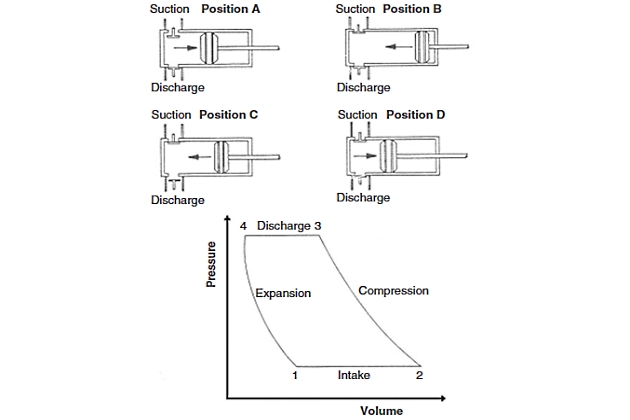
A reciprocating compressor is a positive displacement machine in which the compressing and displacing element is a piston moving linearly within a cylinder. The reciprocating compressor uses automatic spring-loaded valves that open when the proper differential pressure exists across the valve. Figure 1 describes the action of a reciprocating compressor using a theoretical pressure-volume (PV) diagram. In position A, the suction valve is open and gas will flow into the cylinder (from point 1 to point 2 on the PV diagram) until the end of the reverse stroke at point 2, which is the start of compression. At position B, the piston has traveled the full stroke within the cylinder and the cylinder is full of gas at suction pressure. Valves remain closed. The piston begins to move to the left, closing the suction valve. In moving from position B to position C, the piston moves toward the cylinder head, reducing the volume of gas with an accompanying rise in pressure. The PV diagram shows compression from point 2 to point 3. The piston continues to move to the end of the stroke (near the cylinder head) until the cylinder pressure is equal to the discharge pressure and the discharge valve opens (just beyond point 3). After the piston reaches point 4, the discharge valve will close, leaving the clearance space filled with gas at discharge pressure (moving from position C to position D). As the piston reverses its travel, the gas remaining within the cylinder expands (from point 4 to point 1) until it equals suction pressure and the piston is again in position A.

The flow to and from reciprocating compressors is subject to significant pressure fluctuations due to the reciprocating compression process. Therefore, pulsation dampeners have to be installed upstream and downstream of the compressor to avoid damages to other equipment. The pressure losses (several percent of the static flow pressure) of these dampeners have to be accounted for in the station design.

Reciprocating compressors are widely utilized in the gas processing industries because they are flexible in throughput and discharge pressure range. Reciprocating compressors are classified as either “high speed” or “slow speed“. Typically, high-speed compressors operate at speeds of 900 to 1 200 rpm and slow-speed units at speeds of 200 to 600 rpm. High-speed units are normally “separable“, i. e., the compressor frame and driver are separated by a coupling or gearbox. For an “integral” unit, power cylinders are mounted on the same frame as the compressor cylinders, and power pistons are attached to the same drive shaft as the compressor cylinders. Low-speed units are typically integral in design.

Centrifugal Compressors

We want to introduce now the essential components of a centrifugal compressor that accomplish the tasks specified earlier (Figure 2).

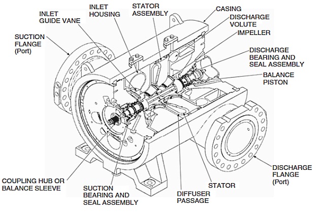
The gas entering the inlet nozzle of the compressor is guided to the inlet of the impeller. An impeller consists of a number of rotating vanes that impart mechanical energy to the gas. The gas will leave the impeller with an increased velocity and increased static pressure. In the diffuser, part of the velocity is converted into static pressure. Diffusers can be vaned, vaneless, or volute type. If the compressor has more than one impeller, the gas will be again brought in front of the next impeller through the return channel and the return vanes. If the compressor has only one impeller, or after the diffuser of the last impeller in a multistage compressor, the gas enters the discharge system. The discharge system can either make use of a volute, which can further convert velocity into static pressure, or a simple cavity that collects the gas before it exits the compressor through the discharge flange.

Read also: The Role of SIGTTO LNG Safety in Advancing Industry Standards

The rotating part of the compressor consists of all the impellers. It runs on two radial bearings (on all modern compressors, these are hydrodynamic tilt pad bearings), while the axial thrust generated by the impellers is balanced by a balance piston, and the resulting force is balanced by a hydrodynamic tilt pad thrust bearing. To keep the gas from escaping at the shaft ends, dry gas seals are used. The entire assembly is contained in a casing (usually barrel type).

A compressor stage is defined as one impeller, with the subsequent diffuser and (if applicable) return channel. A compressor body may hold one or several (up to 8 or 10) stages. A compressor train may consist of one or multiple compressor bodies. It sometimes also includes a gearbox. Pipeline compressors are typically single body trains, with one or two stages.

The different working principles cause differences in the operating characteristics of the centrifugal compressors compared to those of the reciprocating unit. Centrifugal compressors are used in a wide variety of applications in chemical plants, refineries, onshore and offshore gas lift and gas injection applications, gas gathering, and in the transmission of Understanding the Fundamentals of US Natural Gas Pricing and Market Volatilitynatural gas. Centrifugal compressors can be used for outlet pressures as high as 10 000 psia, thus overlapping with reciprocating compressors over a portion of the flow rate/pressure domain. Centrifugal compressors are usually either turbine or electric motor driven. Typical operating speeds for centrifugal compressors in gas transmission applications are about 14 000 rpm for 5 000-hp units and 8 000 rpm for 20 000-hp units.

Comparison Between Compressors

Differences between reciprocating and centrifugal compressors are summarized as follow.

Advantages of a reciprocating compressor over a centrifugal machine include:

• Ideal for low volume flow and high-pressure ratios.
• High efficiency at high-pressure ratios.
• Relatively low capital cost in small units (less than 3 000 hp).
• Less sensitive to changes in composition and density.

Advantages of a centrifugal compressor over a reciprocating machine include:

• Ideal for high volume flow and low head.
• Simple construction with only one moving part.
• High efficiency over normal operating range.
• Low maintenance cost and high availability.
• Greater volume capacity per unit of plot area.
• No vibrations and pulsations generated.

Compressor Selection

The design philosophy for choosing a compressor should include the following considerations.

• Good efficiency over a wide range of operating conditions.
• Maximum flexibility of configuration.
• Low maintenance cost.
• Low life cycle cost.
• Acceptable capital cost.
• High availability.

However, additional requirements and features will depend on each project and on specific experiences of the Pipelines in Marine Terminals: Key Considerations for Handling Liquefied Gaspipeline operator. In fact, compressor selection consists of the purchaser defining the operating parameters for which the machine will be designed. The “process design parameters” that specify a selection are as follows.

1 Flow rate.

2 Gas composition.

3 Inlet pressure and temperature.

4 Outlet pressure.

5 Train arrangement:

• For centrifugal compressors: series, parallel, multiple bodies, multiple sections, intercooling, etc.
• For reciprocating compressors: number of cylinders, cooling, and flow control strategy.

6 Number of units.

In many cases, the decision whether to use a reciprocating compressor or a centrifugal compressor, as well as the type of driver, will already have been made based on operator strategy, emissions requirements, general life cycle cost assumptions, and so on. However, a hydraulic analysis should be made for each compressor selection to ensure the best choice.

In fact, compressor selection can be made for an operating point that will be the most likely or most frequent operating point of the machine. Selections based on a single operating point have to be evaluated carefully to provide sufficient speed margin (typically 3 to 10 %) and surge margin to cover other, potentially important situations. A compressor performance map (for centrifugal compressors, this would be preferably a head vs flow map) can be generated based on the selection and is used to evaluate the compressor for other operating conditions by determining the head and flow required for these other operating conditions. In many applications, multiple operating points are available, e. g., based on hydraulic pipeline studies or reservoir studies. Some of these points may be frequent operating points, while some may just occur during upset conditions. With this knowledge, the selection can be optimized for a desired target, such as lowest fuel consumption.

It will be interesting: Understanding Liquefied Gas Manifolds – Size Categories, Positioning, and Specific Designs for LPG & LNG

Selections can also be made based on a “rated” point, which defines the most onerous operating conditions (highest volumetric flow rate; lowest molecular weight; highest head or pressure ratio; highest inlet temperature). In this situation, however, the result may be an oversized machine that does not perform well at the usual operating conditions.

Once a selection is made, the manufacturer is able to provide parameters such as efficiency, speed, and power requirements and, based on this and the knowledge of the ambient conditions (prevailing temperatures, elevation), can size the drivers. At this point, the casing arrangement and the number of units necessary or desirable (flexibility requirements, growth scenarios and sparing considerations will play an important role in this decision) can be discussed.

Thermodynamics of Gas Compression

The task of gas compression is to bring gas from a certain suction pressure to a higher discharge pressure by means of mechanical work. The actual compression process is often compared to one of three ideal processes: isothermal, isentropic, and polytropic compression.

Isothermal compression occurs when the temperature is kept constant during the compression process. It is not adiabatic because the heat generated in the compression process has to be removed from the system.

The compression process is isentropic or adiabatic reversible if no heat is added to or removed from the gas during compression and the process is frictionless. With these assumptions, the entropy of the gas does not change during the compression process.

The polytropic compression process is like the isentropic cycle reversible, but it is not adiabatic. It can be described as an infinite number of isentropic steps, each interrupted by isobaric heat transfer. This heat addition guarantees that the process will yield the same discharge temperature as the real process.

It is important to clarify certain properties at this time and, in particular, find their connection to the first and second law of thermodynamics written for steady-state fluid flows. The first law (defining the conservation of energy) becomes:

where:

• h – is enthalpy;
• u – is velocity;
• g – is gravitational acceleration;
• z – is elevation coordinate;
• q – is heat;
• and W_t – is work done by the compressor on the gas.

Neglecting the changes in potential energy (because the contribution due to changes in elevation is not significant for Usage of Natural Gas Compressors in the Gas Production Operationsgas compressors), the energy balance equation for adiabatic processes (q₁₂ = 0) can be written as:

W_{t, 12} is the amount of work Physically, there is no difference among work, head, and change in enthalpy. In systems with consistent units (such as the SI system), work, head, and enthalpy difference, have the same unit (e. g., kJ/kg in SI units). Only in inconsistent systems (such as US customary units) do we need to consider that the enthalpy difference (e. g., in Btu/lbm) is related to head and work (e. g., in ft.lbf /lbm) by the mechanical equivalent of heat (e. g., in ft.lbf /Btu).x we have to apply to affect the change in enthalpy in the gas. The work W_{t, 12} is related to the required power, P, by multiplying it with the mass flow.

Combining enthalpy and velocity into a total enthalpy (

$h_t = h + \frac{u^2}{2}$

), power and total enthalpy difference are thus related by:

If we can find a relationship that combines enthalpy with the pressure and temperature of a gas, we have found the necessary tools to describe the gas compression process. For a perfect gas, with constant heat capacity, the relationship among enthalpy, pressures, and temperatures is:

where:

• T1 – is suction temperature;
• T2 – is discharge temperature;
• and C_p – is heat capacity at constant pressure.

For an isentropic compression, the discharge temperature (T_2s) is determined by the pressure ratio as:

where:

• k = C_p/C_v, p₁ – is suction pressure;
• and p₂ – is discharge pressure.

Note that the specific heat at constant pressure (C_p) and the specific heat at constant volume (C_v) are functions of temperature only for ideal gases and can be related together with C_p − C_v = R, where R is the universal gas constant. The isentropic exponent (k) for ideal gas mixtures can also be determined as:

where:

• C_pi – is the molar heat capacity of the individual component;
• and y_i – is the molar concentration of the component.

The heat capacities of real gases are a function of the pressure and temperature and thus may differ from the ideal gas case. For hand calculations, the ideal gas k is sufficiently accurate.

If the Chemical Composition and Physical Properties of Liquefied Gasesgas composition is not known, and the gas is made up of alkanes (such as methane and ethane) with no substantial quantities of contaminants and whose specific gravity (SG) does not exceed unity, the following empirical correlation can be used.

Combining Equations 5 and 6, the isentropic head (∆h_s) for the isentropic compression of a perfect gas can thus be determined as:

For real gases [where k and C_p in Equation 9 become functions of temperature and pressure], the enthalpy of a gas, h, is calculated in a more complicated way using equations of state. These represent relationships that allow one to calculate the enthalpy of gas of known composition if any two of its pressure, its temperature, or its entropy are known.

We therefore can calculate the actual head for the compression by:

and the isentropic head by:

where entropy of the gas at suction condition (s₁) is:

The relationships described can be seen easily in a Mollier diagram (Figure 3).

The performance quality of a compressor can be assessed by comparing the actual head (which relates directly to the amount of power we need to spend for the compression) with the head that the ideal, isentropic compression would require. This defines the isentropic efficiency (η_s) as:

For ideal gases, the actual head can be calculated from:

and further, the actual discharge temperature (T₂) becomes

The second law of thermodynamics tells us:

For adiabatic flows, where no heat q enters or leaves, the change in entropy simply describes the losses generated in the compression process. These losses come from the friction of gas with solid surfaces and the mixing of gas of different energy levels. An adiabatic, reversible compression process therefore does not change the entropy of the system, it is isentropic.

Our equation for the actual head implicitly includes the entropy rise ∆s, because:

If cooling is applied during the compression process (e. g., with intercoolers between two compressors in series), then the increase in entropy is smaller than for an uncooled process. Therefore, the power requirement will be reduced.

Using the polytropic process for comparison reasons works fundamentally the same way as using the isentropic process for comparison reasons. The difference lies in the fact that the polytropic process uses the same discharge temperature as the actual process, while the isentropic process has a different (lower) discharge temperature than the actual process for the same compression task. In particular, both the isentropic and the polytropic processes are reversible processes.

The isentropic process is also adiabatic, whereas the polytropic processes assumes a specific amount of heat transfer. In order to fully define the isentropic compression process for a given gas, suction pressure, suction temperature, and discharge pressure have to be known. To define the polytropic process, in addition either the polytropic compression efficiency or the discharge temperature has to be known. The polytropic efficiency (η_p) is constant for any infinitesimally small compression step, which then allows us to write:

where:

• v – is specific volume, and the polytropic head (∆h_p) can be calculated from:

This determines the polytropic efficiency as:

For compressor designers, the polytropic efficiency has an important advantage. If a compressor has five stages, and each stage has the same isentropic efficiency η_s, then the overall isentropic compressor efficiency will be lower than η_s. If, for the same example, we assume that each stage has the same polytropic efficiency η_p, then the polytropic efficiency of the entire machine is also η_p. As far as performance calculations are concerned, the approach either using a polytropic head and efficiency or using isentropic head and efficiency will lead to the same result:

We also encounter energy conservation on a different level in turbomachines. The aerodynamic function of a turbomachine relies on the capability to trade two forms of energy: kinetic energy (velocity energy) and potential energy (pressure energy), as was outlined earlier.

Real Gas Behavior and Equations of State

Understanding gas compression requires an understanding of the relationship among pressure, temperature, and density of a gas. An ideal gas exhibits the following behavior:

where:

• ρ – is the density of gas;
• and R – is the gas constant.

Any gas at very low pressures (p → 0) can be described by this equation.

For the elevated pressures found in natural gas compression, this equation becomes inaccurate, and an additional variable, the compressibility factor (Z), has to be added:

Unfortunately, the compressibility factor itself is a function of pressure, temperature, and gas composition.

A similar situation arises when the enthalpy has to be calculated. For an ideal gas, we find:

where:

• C_p – is only a function of temperature.

This is a better approximation of the reality than the assumption of a perfect gas used in Equation 5.

In a real gas, we get additional terms for the deviation between real gas behavior and ideal gas behavior:

The terms [h⁰ – h(p₁)]_T1 and [h⁰ – h(p₂)]_T2 are called departure functions because they describe the deviation of real gas behavior from ideal gas behavior. They relate the enthalpy at some pressure and temperature to a reference state at low pressure, but at the same temperature. The departure functions can be calculated solely from an equation of state, while the term ∫ C_pdT is evaluated in the ideal gas state.

Equations of state are semiempirical relationships that allow one to calculate the compressibility factor as well as the departure function. For gas compression applications, the most frequently used equations of state are Redlich – Kwong, Soave – Redlich – Kwong, Benedict – Webb – Rubin, Benedict – Webb – Rubin – Starling and Lee – Kessler – Ploecker.

Kumar et al. and Beinecke and Luedtke have compared these equations of state regarding their accuracy for compression applications. In general, all of these equations provide accurate results for typical applications in pipelines, i. e., for gases with a high methane content, and at pressures below about 3 500 psia. It should be noted that the Redlich-Kwong equation of state is the most effective equation from a computational point of view (because the solution is found directly rather than through an iteration).

Compression Ratio

The compression ratio (CR) is the ratio of absolute discharge pressure to the absolute suction pressure. Mathematically

By definition, the compression ratio is always greater than one. If there are “n” stages of compression and the compression ratio is equal on each stage, then the compression ratio per stage is given by:

If the compression ratio is not equal on each stage, then Equation 26 should be applied to each stage.

The term compression ratio can be applied to a single stage of compression and multistage compression. When applied to a single compressor or a single stage of compression, it is defined as the stage or unit compression ratio; when applied to a multistage compressor it is defined as the overall compression ratio. The compression ratio for typical Velocity Criteria for Sizing Multiphase Pipelinesgas pipeline compressors is rather low (usually below 2), except for stations that feed into pipelines. These low-pressure ratios can be covered in a single compression stage for reciprocating compressor and in a single body (with one or two impellers) in a centrifugal compressor.

While the pressure ratio is a valuable indicator for reciprocating compressors, the pressure ratio that a given centrifugal compressor can achieve depends primarily on gas composition and gas temperature. The centrifugal compressor is better characterized by its capability to achieve a certain amount of head (and a certain amount of head per stage). From Equation 9 it follows that the compressor head translates into a pressure ratio depending on gas composition and suction temperature. For natural gas (SG = 0,58 – 0,65), a single centrifugal stage can provide a pressure ratio of 1,4. The same stage would yield a pressure ratio of about 1,6 if it would compress air (SG = 1,0). The pressure ratio per stage is usually lower than the values given earlier for multistage machines.

Read also: LNG Developments – Key Milestones and Challenges in the Sector

For reciprocating compressors, the pressure ratio per compressor is usually limited by mechanical considerations (rod load) and temperature limitations. Reciprocating compressors can achieve cylinder pressure ratios of 3 to 6. The actual flange-to-flange ratio will be (due to the losses in valves and bottles) lower. For lighter gases (such as natural gas), the temperature limit will often limit the pressure ratio before the mechanical limits do. Centrifugal compressors are also limited by mechanical considerations (rotordynamics, maximum speed) and temperature limits. Whenever any limitation is involved, it becomes necessary to use multiple compression stages in series and intercooling. Furthermore, multistage compression may be required from a purely optimization standpoint. For example, with an increasing compression ratio, compression efficiency decreases and mechanical stress and temperature problems become more severe.

For pressure ratios higher than 3, it may be advantageous to install intercoolers between the compressors. Intercoolers are generally used between the stages to reduce the power requirements as well as to lower the gas temperature that may become undesirably high. After the cooling, liquids may form. These liquids are removed in interstage scrubbers or knockout drums.x Theoretically, a minimum power requirement is obtained with perfect intercooling and no pressure loss between stages by making the ratio of compression the same in all stages. However, intercoolers invariably cause pressure losses (typically between 5 and 15 psi), which is a function of the cooler design.

In the preliminary design, the pressure should be on the order of 10 psi for coolers (especially gas-to-air coolers, where the economics may be out of balance for lower pressure drop).

Note that an actual compressor with an infinite number of compression stages and intercoolers would approach isothermal conditions (where the power requirement of compression cycle is the absolutely minimum power necessary to compress the gas) if the gas were cooled to the initial temperature in the intercoolers.

Interstage cooling is usually achieved using gas-to-air coolers. The gas outlet temperature depends on the ambient air temperature. The intercooler exit temperature is determined by the cooling media. If ambient air is used, the cooler exit temperature, and thus the suction temperature to the second stage, will be about 20 to 30 °F above the ambient dry bulb temperature. Water coolers can achieve exit temperatures about 20 °F above the water supply temperature, but require a constant supply of cooling water. Cooling towers can provide water supply temperatures of about wet bulb temperature plus 25 °F.

For applications where the compressor discharge temperature is above some temperature limit of downstream equipment (a typical example is pipe coatings that limit gas temperatures to about 125 to 140 °F) or has to be limited for other reasons (e. g., to not disturb the permafrost), an aftercooler has to be installed.

Compression design

Compressor design involves several steps. These include selection of the correct type of compressor, as well as the number of stages required. In addition, depending on the capacity, there is also a need to determine the horsepower requirement for the compression.

Determining Number of Stages

For reciprocating compressors, the number of stages is determined from the overall compression ratio as follows.

1. Calculate the overall compression ratio. If the compression ratio is under 4, consider using one stage. If it is not, select an initial number of stages so that CR < 4. For initial calculations it can be assumed that the compression ratio per stage is equal for each stage. Compression ratios of 6 can be achieved for low-pressure applications, however, at the cost of higher mechanical stress levels and lower volumetric efficiency.
2. Calculate the discharge gas temperature for the first stage. If the discharge temperature is too high (more than 300 °F), either increase the number of stages or reduce the suction temperature through precooling. It is recommended that the compressors be sized so that the discharge temperatures for all stages of compression be below 300 °F. It is also suggested that the aerial gas coolers be designed to have a maximum of 20 °F approach to ambient, provided the design reduces the suction temperature for the second stage, conserving horsepower and reducing power demand. If the suction gas temperature to each stage cannot be decreased, increase the number of stages by one and recalculate the discharge temperature.

Note that the 300 °F temperature limit is used for reciprocating compressors because the packing life gets shortened above about 250 °F and the lube oil, being involved directly in the compression process, will degrade faster at higher temperatures. The 350 °F temperature limit pertains to centrifugals and is really a limit for the seals (although special seals can go to 400 to 450 °F) or the pressure rating of casings and flanges. Because the lube oil in a centrifugal compressor does not come into direct contact with the process gas, lube oil degradation is not a factor.

If oxygen is present in the process gas in the amount that it can support combustion (i. e., the gas-to-oxygen ratio is above the lower explosive limit), much lower gas temperatures than mentioned earlier are required.

In reciprocating machines, oil-free compression may be required (no lube oil can come into contact with the process gas). This requires special piston designs that can run dry. Also, a special precaution has to be taken to avoid hot spots generated by local friction.

Inlet Flow Rate

The compressor capacity is a critical component in determining the suitability of a particular compressor. We can calculate the actual gas flow rate While the sizing of the compressor is driven by the actual volumetric flow rate (QG), the flow in many applications is often defined as standard flow. Standard flow is volumetric flow at certain, defined conditions of temperature and pressure (60 °F or 519,7 °R and 14,696 psia) that are usually not the pressures and temperatures of the gas as it enters the compressor.x at suction conditions using:

where:

• Q_G represents an actual cubic feet per minute flow rate of gas;
• T₁ represents the suction temperature in °R;
• p₁ represents suction pressure in psia;
• and Q_{G, SC} represents the standard volumetric flow rate of gas in MMSCFD.

Note that using the value of actual gas volumetric flow rate and discharge pressure, we can roughly determine the type of compressor appropriate for a particular application. Although there is a significant overlap, however, some of the secondary considerations, such as reliability, availability of maintenance, reputation of vendor, and price, will allow one to choose one of the acceptable compressors.

Compression Power Calculation

Once we have an idea about the type of compressor we will select, we also need to know the power requirements so that an appropriate prime mover can be designed for the job. After the gas horsepower (GHP) has been determined by either method, horsepower losses due to friction in bearings, seals, and speed increasing gears must be added. Bearings and seal losses can be estimated from Scheel’s equation. For reciprocating compressors, the mechanical and internal friction losses can range from about 3 to 8 % of the design gas horsepower. For centrifugal compressors, a good estimate is to use 1 to 2 % of the design GHP as mechanical loss.

To calculate brake horsepower (BHP), the following equation can be used.

The detailed calculation of brake horsepower depends on the choice of type of compressor and number of stages. The brake horsepower per stage can be determined from Equation 30:

where:

• BHP – is brake horsepower per stage;
• Z_ave – is average compressibility factor;
• Q_G,SC – is standard volumetric flow rate of gas, MMSCFD;
• T₁ – is suction temperature, ◦R;
• p₁, p₂ are pressure at suction and discharge flanges, respectively, psia;
• E – is parasitic efficiency (for high-speed reciprocating units, use 0,72 to 0,82; for low-speed reciprocating units, use 0,72 to 0,85; and for centrifugal units, use 0,99);
• η – is compression efficiency (1,0 for reciprocating and 0,80 to 0,87 for centrifugal units).

In Equation 30, parasitic efficiency (E) accounts for mechanical losses, and the pressure losses incurred in the valves and pulsation dampeners of reciprocating compressors (the lower efficiencies are usually associated with low-pressure ratio applications typical for pipeline compression). Many calculation procedures for reciprocating compressors use numbers for E that are higher than the ones referenced here. These calculations require, however, that the flange-to-flange pressure ratio [which is used in Equation 30] is increased by the pressure losses in the compressor suction and discharge valves, and pulsation dampeners. These pressure losses are significant, especially for low head, high flow applications.x

Hence, suction and discharge pressures may have to be adjusted for the pressure losses incurred in the pulsation dampeners for reciprocation compressors. The compression efficiency accounts for the actual compression process. For centrifugal compressors, the lower efficiency is usually associated with pressure ratios of 3 and higher. Very low flow compressors (below 1 000 acfm) may have lower efficiencies.

It will be interesting: Comprehensive Guide to Local Content Policies and Infrastructure Development

The total horsepower for the compressor is the sum of the horsepower required for each stage. Reciprocating compressors require an allowance for interstage pressure losses. It can be assumed that there is a 3 % loss of pressure in going through the cooler, scrubbers, piping, and so on between the actual discharge of the cylinder and the actual suction of the next cylinder. For a centrifugal compressor, any losses incurred between the stages are already included in the stage efficiency. However, the exit temperature from the previous stage becomes the inlet temperature in the next stage. If multiple bodies are used, the losses for coolers and piping have to be included as described previously.

Example

Given the following information for a centrifugal compressor, answer the following questions.

Operating Conditions

• P_s = 750 psia;
• P_d = 1046,4 psia;
• T_s = 529,7 °R;
• T_d = 582,6 °R;
• Q_{G, SC} = 349 MMSCFD.

Gas Properties

• SG = 0,6;
• k = 1,3;
• Z_ave = 0,95

Questions

1. What is the isentropic efficiency?
2. What is the actual volumetric flow rate?
3. What is the isentropic head?
4. What is the power requirement (assume a 98 % mechanical efficiency)?

Solution

1 With rearranging Equation 15, we find:

2 Mass flow is:

and thus the volumetric flow becomes

3 The isentropic head follows from Equation 9 with C_p = (53,35/SG) Z k/(k−1)

4 The power can be calculated from Equation 30

Compressor Control

To a large extent, the compressor operating point will be the result of the pressure conditions imposed by the system. However, the pressures imposed by the system may in turn be dependent on the flow. Only if the conditions fall outside the operating limits of the compressor (e. g., frame loads, discharge temperature, available driver power, surge, choke, speed), do control mechanisms have to be in place. However, the compressor output may have to be controlled to match the system demand.

The type of application often determines the system behavior. In a pipeline application, suction and discharge pressure are connected with the flow by the fact that the more flow is pushed through a pipeline, the more pressure ratio is required at the compressor station to compensate for the pipeline pressure losses. In processelated applications, the suction pressure may be fixed by a back pressure-controlled production separator.

In boost applications, the discharge pressure is determined by the pressure level of the pipeline the compressor feeds into, whereas the suction pressure is fixed by the process. In oil and gas field applications, the suction pressure may depend on the flow because the more gas is moved out of the gas reservoir, the lower the suction pressure has to be. The operation may require constant flow despite changes in suction or discharge pressure. Compressor flow, pressure, or speed may have to be controlled.

The type of control also depends on the compressor driver. Both reciprocating compressors and centrifugal compressors can be controlled by suction throttling or recirculating of gas. However, either method is very inefficient for process control (but may be used to protect the compressor) because the reduction in flow or head is not accompanied by a significant reduction in the power requirement.

Reciprocating Compressors

The following mechanisms may be used to control the capacity of reciprocating compressors:

• suction pressure,
• variation of clearance,
• speed,
• valve unloading,
• and recycle.

Reciprocating compressors tend to have a rather steep head versus flow characteristic. This means that changes in pressure ratio have a very small effect on the actual flow through the machine.

Read also: Mastering Natural Gas Fundamentals Properties Sources and Transport Insights

Controlling the flow through the compressor can be accomplished by varying the operating speed of the compressor. This method can be used if the compressor is driven by an internal combustion engine or a variable speed electric motor. Internal combustion engines, along with variable speed electric motors, produce less power if they operate at a speed different from their optimum speed. Internal combustion engines allow for speed control in the range of 70 to 100 % of maximum speed.

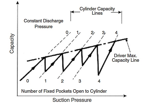
If the driver is a constant speed electric motor, the capacity control consists of either inlet valve unloaders or clearance unloaders. Inlet valve unloaders can hold the inlet valve into the compressor open, thereby preventing compression. Clearance unloaders consist of pockets that are opened when unloading is desired. The gas is compressed into them at the compression stroke and expands back into the cylinder on the return stroke, thus reducing the intake of additional gas and subsequently the compressor capacity. Additional flexibility is achieved using several steps of clearance control and combinations of clearance control and inlet valve control. Figure 4 shows the control characteristic of such a compressor.

Reciprocating compressors generate flow pulsations in the suction and discharge lines that have to be controlled to prevent over- and underloading of the compressors, to avoid vibration problems in the piping or other machinery at the station, and to provide a smooth flow of gas. Flow pulsations can be reduced greatly by properly sized pulsation bottles or pulsation dampeners in the suction and discharge lines.

Centrifugal Compressors

As with reciprocating compressors, the compressor output must be controlled to match the system demand. The operation may require constant flow despite changes in suction or discharge pressure. Compressor flow, pressure, or speed may have to be controlled. The type of control also depends on the compressor driver. Centrifugal compressors tend to have a rather flat head versus flow characteristic. This means that changes in pressure ratio have a significant effect on the actual flow through the machine.

Compressor control is usually accomplished by speed control, variable guide vanes, suction throttling, and recycling of gas. Only in rare cases are adjustable diffuser vanes used. To protect the compressor from surge, recycling is used. Controlling the flow through the compressor can be accomplished by varying the operating speed of the compressor. This is the preferred method of controlling centrifugal compressors. Two shaft gas turbines and variable speed electric motors allow for speed variations over a wide range (usually from 50 to 100 % of maximum speed or more).

Virtually any centrifugal compressor installed since the early 1990s in pipeline service is driven by variable speed drivers, usually a two-shaft gas turbine. Older installations and installations in other than pipeline services sometimes use single shaft gas turbines (which allow a speed variation from about 90 to 100 % speed) and constant speed electric motors. In these installation, suction throttling or variable inlet guide vanes are used to provide means of control.

The operating envelope of a centrifugal compressor is limited by the maximum allowable speed, the minimum allowable speed, the minimum flow (surge flow), and the maximum flow (choke or stonewall) (Figure 5).

Another limiting factor may be the available driver power. Only the minimum flow requires special attention because it is defined by an aerodynamic stability limit of the compressor. Crossing this limit to lower flows will cause pulsating intermittent flow reversals in the compressor (surge), which eventually can damage the compressor. Modern control systems can detect this situation and shut the machine down or prevent it entirely by automatically opening a recycle valve. For this reason, virtually all modern compressor installations use a recycle line (Figure 6) with a control valve that allows the flow to increase through the compressor if it comes near the stability limit. Modern control systems constantly monitor the operating point of the compressor in relation to its surge line and automatically open or close the recycle valve if necessary.

The control system is designed to compare the measured operating point of the compressor with the position of the surge line (Figure 5). To that end, flow, suction pressure, discharge pressure, and suction temperature, as well as compressor speed, have to be measured.

Compressor Performance Maps

Reciprocating Compressors

Figure 7 shows some typical performance maps for reciprocating compressors.

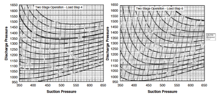
Because the operating limitations of a reciprocating compressor are often defined by mechanical limits (especially maximum rod load) and because the pressure ratio of the machine is very insensitive to changes in suction conditions and gas composition, we usually find maps depicting suction and discharge pressures and actual flow. Maps account for the effect of opening or closing pockets and for variations in speed.

Centrifugal Compressors

For a centrifugal compressor, the head (rather than the pressure ratio) is rather invariant with the change in suction conditions and gas composition. As with the reciprocating compressor, the flow that determines the operating point is the actual flow as opposed to mass flow or standard flow.

Head versus actual flow maps (Figure 5) are therefore the most usual way to describe the operating range of a centrifugal compressor.

It will be interesting: Phase Separation: An Essential Process in Hydrocarbon Production

These maps change very little even if the inlet conditions or the gas composition changes. They depict the effect of changing the operating speed and define the operating limits of the compressor, such as surge limit, maximum and minimum speed, and maximum flow at choke conditions. Every set of operating conditions, given as suction pressure, discharge pressure, suction temperature, flow, and gas composition, can be converted into isentropic head and actual flow using the relationships described previously. Once the operating point is located on a head flow map, the efficiency of the compressor, and the required operating speed, as well as the surge margin, can be determined.

Author

Olga Nesvetailova

Freelancer

Literature

1. Acikgoz, M., Franca, F., and Lahey Jr, R. T., An experimental study of three-phase flow regimes. Int. J. Multiphase Flow 18(3), 327-336 (1992).
2. Adewmi, M. A., and Bukacek, R. F., Two-phase pressure drop in horizontal pipelines. J. Pipelines 5, 1-14 (1985).
3. Amdal, J., et al., “Handbook of Multiphase Metering.” Produced for The Norwegian Society for Oil and Gas Measurement, Norway (2001).
4. Ansari, A. M., Sylvester, A. D., Sarica, C., Shoham, O., and Brill, J. P., A comprehensive mechanistic model for upward two-phase flow in wellbores. SPE Prod. Facilit. J. 143-152 (May 1994).
5. API, “Computational Pipeline Monitoring”. API Publication 1130, 17, American Petroleum Institute, TX (1995a).
6. API, “Evaluation Methodology for Software Based Leak Detection Systems”. API Publication 1155, 93, American Petroleum Institute, TX (1995b).
7. API RP 14E, “Recommended Practice for Design and Installation of Offshore Production Platform Piping Systems”, 5th Ed., p. 23.
8. Asante, B., “Two-Phase Flow: Accounting for the Presence of Liquids in Gas Pipeline Simulation”. Paper presented at 34th PSIG Annual Meeting, Portland, Oregon (Oct. 23–25, 2002).
9. AsphWax’s Flow Assurance course, “Fluid Characterization for Flow Assurance”. AsphWax Inc., Stafford, TX (2003).
10. Ayala, F. L., and Adewumi, M. A., Low-liquid loading multiphase flow in natural gas pipelines. ASME J. of Energy Res. Technol. 125, 284-293 (2003).
11. Baillie, C., and Wichert, E., Chart gives hydrate formation temperature for natural gas. Oil Gas J. 85(4), 37-39 (1987).
12. Baker, O., Design of pipelines for simultaneous flow of oil and gas. Oil Gas J. 53, 185 (1954).
13. Banerjee, S., “Basic Equations”. Lecture presented at the Short Course on Modeling of Two-Phase Flow Systems, ETH Zurich, Switzerland (March 17-21, 1986).
14. Barnea, D., A unified model for prediction flow pattern transitions for the whole range of pipe inclinations. Int. J. Multiphase Flow 13(1), 1-12 (1987).
15. Barnea, D., and Taitel, Y., Stratified three-phase flow in pipes: Stability and transition. Chem. Eng. Comm. 141–142, 443-460 (1996).
16. Battara, V., Gentilini, M., and Giacchetta, G., Condensate-line correlations for calculating holdup, friction compared to field data. Oil Gas J. 30, 148–52 (1985).
17. Bay, Y., “Pipelines and Risers”, Vol. 5. Elsevier Ocean Engineering Book Series (2001).
18. Beggs, H. D., and Brill, J. P., “A Study of Two-Phase Flow in Inclined Pipes”. JPT, 607-17; Trans., AIME, 255 (May 1973).
19. Bendiksen, K., Brandt, I., Jacobsen, K. A., and Pauchon, C., “Dynamic Simulation of Multiphase Transportation Systems”. Multiphase Technology and Consequence for Field Development Forum, Stavanger, Norway (1987).
20. Bendiksen, K., Malnes, D., Moe, R., and Nuland, S., The dynamic two-fluid model OLGA: Theory and application. SPE Prod. Eng. 6, 171-180 (1991).
21. Bertola, V., and Cafaro, E., “Statistical Characterization of Subregimes in Horizontal Intermittent Gas/Liquid Flow”. Proc. the 4th International Conference on Multiphase Flow, New Orleans, LA (2001).
22. Bjune, B., Moe, H., and Dalsmo, M., Upstream control and optimization increases return on investment. World Oil 223, 9 (2002).
23. Black, P. S., Daniels, L. C., Hoyle, N. C., and Jepson, W. P., Studying transient multiphase flow using the pipeline analysis code (PLAC). ASME J. Energy Res. Technol. 112, 25-29 (1990).
24. Bloys, B., Lacey, C., and Lynch, P., “Laboratory Testing and Field Trial of a New Kinetic Hydrate Inhibitor”. Proc. 27th Annual Offshore Technology Conference, OTC 7772, PP. 691-700, Houston, TX (1995).
25. Bonizzi, M., and Issa, R. I., On the simulation of three-phase slug flow in nearly horizontal pipes using the multi-fluid model. Int. J. Multiphase Flow 29, 1719-1747 (2003).
26. Boriyantoro, N. H., and Adewumi, M. A., “An Integrated Single-Phase/Two-Phase Flow Hydrodynamic Model for Predicting the Fluid Flow Behavior of Gas Condensate Pipelines”. Paper presented at 26th PSIG Annual Meeting, San Diego, CA (1994).
27. Brauner, N., and Maron, M. D., Flow pattern transitions in two-phase liquid-liquid flow in horizontal tubes, Int. J. Multiphase Flow 18, 123-140 (1992).
28. Brauner, N., The prediction of dispersed flows boundaries in liquid-liquid and gas-liquid systems, Int. J. Multiphase Flow 27, 885-910 (2001).
29. Brill, J. P., and Beggs, H. D., “Two-Phase Flow in Pipes”, 6th Ed. Tulsa University Press, Tulsa, OK (1991).
30. Bufton, S. A., Ultra Deepwater will require less conservative flow assurance approaches. Oil Gas J. 101(18), 66-77 (2003).
31. Campbell, J. M., “Gas Conditioning and Processing”, 3rd Ed. Campbell Petroleum Series, Norman, OK (1992).
32. Carroll, J. J., “Natural Gas Hydrates: A Guide for Engineers”. Gulf Professional Publishing, Amsterdam, The Netherlands (2003).
33. Carroll, J. J., “An Examination of the Prediction of Hydrate Formation Conditions in Sour Natural Gas”. Paper presented at the GPA Europe Spring Meeting, Dublin, Ireland (May 19-21, 2004).
34. Carson, D. B., and Katz, D. L., Natural gas hydrates. Petroleum Trans. AIME 146, 150-158 (1942).
35. Chen, C. J., Woo, H. J., and Robinson, D. B., “The Solubility of Methanol or Glycol in Water-Hydrocarbon Systems”. GPA Research Report RR-117, Gas Processors Association, OK (March 1988).
36. Chen, X., and Guo, L., Flow patterns and pressure drop in oil-air-water three-phase flow through helically coiled tubes. Int. J. Multiphase Flow 25, 1053-1072 (1999).
37. Cheremisinoff, N. P., “Encyclopedia of Fluid Mechanics”, Vol. 3. Gulf Professional Publishing, Houston, TX (1986).
38. Chisholm, D., and Sutherland, L. A., “Prediction of Pressure Gradient in Pipeline Systems during Two-Phase Flow”. Paper presented at Symposium on Fluid Mechanics and Measurements in Two-Phase Flow Systems, Leeds (Sept. 1969).
39. Cindric, D. T., Gandhi, S. L., and Williams, R. A., “Designing Piping Systems for Two-Phase Flow”. Chem. Eng. Progress, 51-59 (March 1987).
40. Collier, J. G., and Thome, J. R., “Convective Boiling and Condensation”, 3rd Ed. Clarendon Press, Oxford, UK (1996).
41. Colson, R., and Moriber, N. J., Corrosion control. Civil Eng. 67(3), 58-59 (1997).
42. Copp, D. L., “Gas Transmission and Distribution”. Walter King Ltd., London (1970).
43. Courbot, A., “Prevention of Severe Slugging in the Dunbar 16 Multiphase Pipelines”. Paper presented at the Offshore Technology Conference, Houston, TX (May 1996).
44. Covington, K. C., Collie, J. T., and Behrens, S. D., “Selection of Hydrate Suppression Methods for Gas Streams”. Paper presented at the 78th GPA Annual Convention, Nashville, TN (1999).
45. Cranswick, D., “Brief Overview of Gulf of Mexico OCS Oil and Gas Pipelines: Installation, Potential Impacts, and Mitigation Measures”. U. S. Department of the Interior, Minerals Management Service, Gulf of Mexico OCS Region, New Orleans, LA (2001).
46. Dhl, E., et al., “Handbook of Water Fraction Metering”, Rev. 1. Norwegian Society for Oil and Gas Measurements, Norway (June 2001).
47. Decarre, S., and Fabre, J., Etude Sur La Prediction De l’Inversion De Phase. Revue De l’Institut Francais Du Petrole 52, 415-424 (1997).
48. De Henau, V., and Raithby, G. D., A transient two-fluid model for the simulation of slug flow in pipelines. Int. J. Multiphase Flow 21, 335–349 (1995).
49. Dukler, A. E., “Gas-Liquid Flow in Pipelines Research Results”. American Gas Assn. Project NX-28 (1969).
50. Dukler, A. E., and Hubbard, M. G., “The Characterization of Flow Regimes for Horizontal Two-Phase Flow”. Proc. Heat Transfer and Fluid Mechanics Institute, 1, 100-121, Stanford University Press, Stanford, CA (1966).
51. Eaton, B. A., et al., The prediction of flow pattern, liquid holdup and pressure losses occurring during continuous two-phase flow in horizontal pipelines. J. Petro. Technol. 240, 815-28 (1967).
52. Edmonds, B., et al., “A Practical Model for the Effect of Salinity on Gas Hydrate Formation”. European Production Operations Conference and Exhibition, Norway (April 1996).
53. Edmonds, B., Moorwood, R. A. S., and Szczepanski, R., “Hydrate Update”. GPA Spring Meeting, Darlington (May 1998).
54. Esteban, A., Hernandez, V., and Lunsford, K., “Exploit the Benefits of Methanol”. Paper presented at the 79th GPA Annual Convention, Atlanta, GA (2000).
55. Fabre, J., et al., Severe slugging in pipeline/riser systems. SPE Prod. Eng. 5(3), 299-305 (1990).
56. Faille, I., and Heintze, E., “Rough Finite Volume Schemes for Modeling Two-Phase Flow in a Pipeline”. In Proceeding of the CEA.EDF.INRIA Course, INRIA Rocquencourt, France (1996).
57. Fidel-Dufour, A., and Herri, J. S., “Formation and Dissociation of Hydrate Plugs in a Water in Oil Emulsion”. Paper presented at the 4th International Conference on Gas Hydrates, Yokohama, Japan (2002).
58. Frostman, L. M., “Anti-aggolomerant Hydrate Inhibitors for Prevention of Hydrate Plugs in Deepwater Systems”. Paper presented at the SPE Annual Technical Conference and Exhibition, Dallas, TX (Oct. 1-4, 2000).
59. Frostman, L. M., et al., “Low Dosage Hydrate Inhibitors (LDHIs): Reducing Total Cost of Operations in Existing Systems and Designing for the Future”. Paper presented at the SPE International Symposium on Oilfield Chemicals, Houston, TX (Feb. 5-7, 2003).
60. Frostman, L. M., “Low Dosage Hydrate Inhibitor (LDHI) Experience in Deepwater”. Paper presented at the Deep Offshore Technology Conference, Marseille, France (Nov. 19-21, 2003).
61. Fuchs, P., “The Pressure Limit for Terrain Slugging”. Proceeding of the 3rd BHRA International Conference on Multiphase Flow, Hague, The Netherlands (May 1987).
62. Furlow, W., “Suppression System Stabilizes Long Pipeline-Riser Liquid Flows”. Offshore, Deepwater D&P, 48 + 166 (Oct., 2000).
63. Giot, M., “Three-Phase Flow”, Chap. 7.2. McGraw-Hill, New York (1982).
64. Goulter, D., and Bardon, M., Revised equation improves flowing gas temperature prediction. Oil Gas J. 26, 107-108 (1979).
65. Govier, G. W., and Aziz, K., “The Flow of Complex Mixtures in Pipes”. Van Nostrand Reinhold Co., Krieger, New York (1972).
66. GPSA Engineering Data Book, 11th Ed. Gas Processors Suppliers Association, Tulsa, OK (1998).
67. Gregory, G. A., and Aziz, K., Design of pipelines for multiphase gas-condensate flow. J. Can. Petr. Technol. 28-33 (1975).
68. Griffith, P., and Wallis, G. B., Two-phase slug flow. J. Heat Transfer Trans. ASME. 82, 307-320 (1961).
69. Haandrikman, G., Seelen, R., Henkes, R., and Vreenegoor, R., “Slug Control in Flowline/Riser Systems”. Paper presented at the 2nd International Conference on Latest Advance in Offshore Processing, Aberdeen, UK (Nov. 9-10, 1999).
70. Hall, A. R. W., “Flow Patterns in Three-Phase Flows of Oil, Water, and Gas”. Paper presented at the 8th BHRG International Conference on Multiphase Production, Cannes, France (1997).
71. Hammerschmidt, E. G., Formation of gas hydrates in natural gas transmission lines. Ind. Eng. Chem. 26, 851-855 (1934).
72. Hart, J., and Hamersma P. J. Correlations predicting frictional pressure drop and liquid holdup during horizontal gas-liquid pipe flow with small liquid holdup. Int. J. Multiphase Flow 15(6), 974-964 (1989).
73. Hartt, W. H., and Chu, W., New methods for CP design offered. Oil Gas J. 102(36), 64-70 (2004).
74. Hasan, A. R., Void fraction in bubbly and slug flow in downward two-phase flow in vertical and inclined wellbores, SPE Prod. Facil. 10(3), 172–176 (1995).
75. Hasan, A. R., and Kabir, C. S., “Predicting Multiphase Flow Behavior in a Deviated Well”. Paper presented at the 61st SPE Annual Technical Conference and Exhibition, New Orleans, LA (1986).
76. Hasan, A. R., and Kabir, C. S., Gas void fraction in two-phase up-flow in vertical and inclined annuli. Int. J. Multiphase Flow 18(2), 279-293 (1992).
77. Hasan, A. R., and Kabir, C. S., Simplified model for oil/water flow in vertical and deviated wellbores. SPE Prod. Facil. 14(1), 56-62 (1999).
78. Hasan, A. R., and Kabir, C. S., “Fluid and Heat Transfers in Wellbores”. Society of Petroleum Engineers (SPE) Publications, Richardson, TX (2002).
79. Havre, K., and Dalsmo, M., “Active Feedback Control as the Solution to Severe Slugging”. Paper presented at the SPE Annual Technical Conference and Exhibition, New Orleans, LA (Oct. 3, 2001).
80. Havre, K., Stornes, K., and Stray, H., “Taming Slug Flow in Pipelines”. ABB Review No. 4, 55-63, ABB Corporate Research AS, Norway (2000).
81. Hedne, P., and Linga, H., “Suppression of Terrain Slugging with Automatic and Manual Riser Chocking”. Advances in Gas-Liquid Flows, 453-469 (1990).
82. Hein, M., “HP41 Pipeline Hydraulics and Heat Transfer Programs.” PennWell Publishing Company, Tulsa, OK (1984).
83. Henriot, V., Courbot, A., Heintze, E., and Moyeux, L., “Simulation of Process to Control Severe Slugging: Application to the Dunbar Pipeline”. Paper presented at the SPE Annual Conference and Exhibition, Houston, TX (1999).
84. Hewitt, G. F., and Roberts, D. N., “Studies of Two-Phase Flow Patterns by Simultaneous X-ray and Flash Photography”. AERE-M 2159, HMSO (1969).
85. Hill, T. H., Gas injection at riser base solves slugging, flow problems. Oil Gas J. 88(9), 88-92 (1990).
86. Hill, T. J., “Gas-Liquid Challenges in Oil and Gas Production”. Proceeding of ASME Fluids Engineering Division Summer Meeting, Vancouver, BC, Canada (June 22-26, 1997).
87. Holt, A. J., Azzopardi, B. J., and Biddulph, M. W., “The Effect of Density Ratio on Two-Phase Frictional Pressure Drop”. Paper presented at the 1st International Symposium on Two-Phase Flow Modeling and Experimentation, Rome, Italy (Oct. 9-11, 1995).
88. Holt, A. J., Azzopardi, B. J., and Biddulph, M. W., Calculation of two-phase pressure drop for vertical up flow in narrow passages by means of a flow pattern specific models. Trans. IChemE 77(Part A), 7-15 (1999).
89. Hunt, A., Fluid properties determine flow line blockage potential. Oil Gas J. 94(29), 62–66 (1996).
90. IFE, “Mitigating Internal Corrosion in Carbon Steel Pipelines”. Institute of Energy Technology News, Norway (April 2000).
91. Jansen, F. E., Shoham, O., and Taitel, Y., The elimination of severe slug-ging, experiments and modeling. Int. J. Multiphase Flow 22(6), 1055-1072 (1996).
92. Johal, K. S., et al., “An Alternative Economic Method to Riser Base Gas Lift for Deepwater Subsea Oil/Gas Field Developments”. Proceeding of the Offshore Europe Conference, 487-492, Aberdeen, Scotland (9-12 Sept., 1997).
93. Jolly, W. D., Morrow, T. B., O’Brien, J. F., Spence, H. F., and Svedeman, S. J., “New Methods for Rapid Leak Detection in Offshore Pipelines”. Final Report, SWRI Project No. 04-4558, SWRI (April 1992).
94. Jones, O. C., and Zuber, N., The interrelation between void fraction fluctuations and flow patterns in two-phase flow Int. J. Multiphase Flow. 2, 273-306 (1975).
95. Kang, C., Wilkens, R. J., and Jepson, W. P., “The Effect of Slug Frequency on Corrosion in High-Pressure, Inclined Pipelines”. Paper presented at the NACE International Annual Conference and Exhibition, Paper No. 96020, Denver, CO (March 1996).
96. Katz, D. L., Prediction of conditions for hydrate formation in natural gases. Trans. AIME 160, 140–149 (1945).
97. Kelland, M. A., Svartaas, T. M., and Dybvik, L., “New Generation of Gas Hydrate Inhibitors”. 70th SPE Annual Technical Conference and Exhibition, 529-537, Dallas, TX (Oct. 22-25, 1995).
98. Kelland, M. A., Svartaas, T. M., Ovsthus, J., and Namba, T., A new class of kinetic inhibitors. Ann. N. Y. Acad. Sci. 912, 281-293 (2000).
99. King, M. J. S, “Experimental and Modelling Studies of Transient Slug Flow”. Ph.D. Thesis, Imperial College of Science, Technology, and Medicine, London, UK (March 1998).
100. Klemp, S., “Extending the Domain of Application of Multiphase Technology”. Paper presented at the 9th BHRG International Conference on Multiphase Technology, Cannes, France (June 16-18, 1999).
101. Kohl, A. L., and Risenfeld, F. C., “Gas Purification.” Gulf Professional Publishing, Houston, TX (1985).
102. Kovalev, K., Cruickshank, A., and Purvis, J., “Slug Suppression System in Operation”. Paper presented at the 2003 Offshore Europe Conference, Aberdeen, UK (Sept. 2-5, 2003).
103. Kumar, S., “Gas Production Engineering”. Gulf Professional Publishing, Houston, TX (1987).
104. Lagiere, M., Miniscloux, and Roux, A., Computer two-phase flow model predicts pipeline pressure and temperature profiles. Oil Gas J. 82-91 (April 9, 1984).
105. Langner, et al., “Direct Impedance Heating of Deepwater Flowlines.” Paper presented at the Offshore Technology Conference (OTC), Houston, TX (1999).
106. Lederhos, J. P., Longs, J. P., Sum, A., Christiansen, R. l., and Sloan, E. D., Effective kinetic inhibitors for natural gas hydrates. Chem. Eng. Sci. 51(8), 1221-1229 (1996).
107. Lee, H. A., Sun, J. Y., and Jepson, W. P., “Study of Flow Regime Transitions of Oil-Water-Gas Mixture in Horizontal Pipelines”. Paper presented at the 3rd International Offshore and Polar Engng Conference, Singapore (June 6–11 1993).
108. Leontaritis, K. J., “The Asphaltene and Wax Deposition Envelopes”. The Symposium on Thermodynamics of Heavy Oils and Asphaltenes, Area 16C of Fuels and Petrochemical Division, AIChE Spring National Meeting and Petroleum Exposition, Houston, TX (March 19-23, 1995).
109. Leontaritis, K. J., “PARA-Based (Paraffin-Aromatic-Resin-Asphaltene) Reservoir Oil Characterization”. Paper presented at the SPE International Symposium on Oilfield Chemistry, Houston, TX (Feb. 18-21, 1997a).
110. Leontaritis, K. J., Asphaltene destabilization by drilling/completion fluids. World Oil 218(11), 101-104 (1997b).
111. Leontaritis, K. J., “Wax Deposition Envelope of Gas Condensates”. Paper presented at the Offshore Technology Conference (OTC), Houston, TX (May 4–7 1998).
112. Lin, P. Y., and Hanratty, T. J., Detection of slug flow from pressure measurements. Int. J. Multiphase Flow 13, 13-21 (1987).
113. Lockhart, R. W., and Martinelli, R. C., Proposed correlation of data for isothermal two-phase, two-component flow in pipes. Chem. Eng. Prog. 45, 39-48 (1949).
114. Maddox, R. N., et al., “Predicting Hydrate Temperature at High Inhibitor Concentration”. Proceedings of the Laurance Reid Gas Conditioning Conference, 273-294, Norman, OK (1991).
115. Mann, S. L., et al., “Vapour-Solid Equilibrium Ratios for Structure I and II Natural Gas Hydrates”. Proceedings of the 68th GPA Annual Convention, 60-74, San Antonio, TX (March 13-14, 1989).
116. Martinelli, R. C., and Nelson, D. B., Prediction of pressure drop during forced circulation boiling of water. Trans. ASME 70, 695 (1948).
117. Masella, J. M., Tran, Q. H., Ferre, D., and Pauchon, C., Transient simulation of two-phase flows in pipes. Oil Gas Sci. Technol. 53(6), 801–811 (1998).
118. McCain, W. D., “The Properties of Petroleum Fluids”, 2nd Ed. Pennwell Publishing Company, Tulsa, OK (1990).
119. McLaury, B. S., and Shirazi, S. A., An alternative method to API RP 14E for predicting solids erosion in multiphase flow. ASME J. Energy Res. Technol. 122, 115-122 (2000).
120. McLeod, H. O., and Campbell, J. M., Natural gas hydrates at pressure to 10,000 psia. J. Petro. Technol. 13, 590-594 (1961).
121. Mehta, A. P., and Sloan, E. D., “Structure H Hydrates: The State-of-the-Art”. Paper presented at the 75th GPA Annual Convention, Denver, CO (1996).
122. Mehta, A., Hudson, J., and Peters, D., “Risk of Pipeline Over-Pressurization during Hydrate Remediation by Electrical Heating”. Paper presented at the Chevron Deepwater Pipeline and Riser Conference, Houston, TX (March 28-29, 2001).
123. Mehta, A. P., Hebert, P. B., and Weatherman, J. P., “Fulfilling the Promise of Low Dosage Hydrate Inhibitors: Journey from Academic Curiosity to Successful Field Implementations”. Paper presented at the 2002 Offshore Technology Conference, Houston, TX (May 6-9, 2002).
124. Minami, K., “Transient Flow and Pigging Dynamics in Two-Phase Pipelines”. Ph.D. Thesis, University of Tulsa, Tulsa, OK (1991).
125. Mokhatab, S., Correlation predicts pressure drop in gas-condensate pipelines. Oil Gas J. 100(4), 66-68 (2002a).
126. Mokhatab, S., New correlation predicts liquid holdup in gas-condensate pipelines. Oil Gas J. 100(27), 68-69 (2002b).
127. Mokhatab, S., Model aids design of three-phase, gas-condensate transmission lines. Oil Gas J. 100(10), 60-64 (2002c).
128. Mokhatab, S., Three-phase flash calculation for hydrocarbon systems containing water. J. Theor. Found. Chem. Eng. 37(3), 291-294 (2003).
129. Mokhatab, S., Upgrade velocity criteria for sizing multiphase pipelines. J. Pipeline Integrity 3(1), 55-56 (2004).
130. Mokhatab, S., “Interaction between Multiphase Pipelines and Down-stream Processing Plants”. Report No. 3, TMF3 Sub-Project VII: Flexible Risers, Transient Multiphase Flow (TMF) Program, Cranfield University, Bedfordshire, England (May 2005).
131. Mokhatab, S., “Explicit method predicts temperature and pressure profiles of gas-condensate pipelines”. Accepted for publication in Energy Sources: Part A (2006a).
132. Mokhatab, S., Severe slugging in a catenary-shaped riser: Experimental and simulation studies”. Accepted for publication in J. Petr. Sci. Technol. (2006b).
133. Mokhatab, S., Dynamic simulation of offshore production plants. Accepted for publication in J. Petr. Sci. Technol. (2006c).
134. Mokhatab, S., Severe slugging in flexible risers: Review of experimental investigations and OLGA predictions. Accepted for publication in J. Petro. Sci. Technol. (2006d).
135. Mokhatab, S., and Bonizzi, M., “Model predicts two-phase flow pressure drop in gas-condensate transmission lines”. Accepted for publication in Energy Sources: Part A (2006).
136. Mokhatab, S., Towler, B. F., and Purewal, S., A review of current technologies for severe slugging remediation”. Accepted for publication in J. Petro. Sci. Technol. (2006a).
137. Mokhatab, S., Wilkens, R. J., and Leontaritis, K. J., “A Review of strategies for solving gas hydrate problems in subsea pipelines”. Accepted for publication in Energy Sources: Part A (2006b).
138. Molyneux, P., Tait, A., and Kinving, J., “Characterization and Active Control of Slugging in a Vertical Riser”. Proceeding of the 2nd North American Conference on Multiphase Technology, 161–170, Banff, Canada (June 21–23, 2000).
139. Moody, L. F., Friction factors for pipe flow. Trans. ASME 66, 671–684 (1944).
140. Mucharam, L., Adewmi, M. A., and Watson, R., Study of gas condensation in transmission pipelines with a hydrodynamic model. SPE J. 236–242 (1990).
141. Muhlbauer, K. W., “Pipeline Risk Management Manual”, 2nd Ed. Gulf Professional Publishing, Houston, TX (1996).
142. Narayanan, L., Leontaritis, K. J., and Darby, R., “A Thermodynamic Model for Predicting Wax Precipitation from Crude Oils”. The Symposium of Solids Deposition, Area 16C of Fuels and Petro-chemical Division, AIChE Spring National Meeting and Petroleum Exposition, Houston, TX (March 28-April 1, 1993).
143. Nasrifar, K., Moshfeghian, M., and Maddox, R. N., Prediction of equilibrium conditions for gas hydrate formation in the mixture of both electrolytes and alcohol. Fluid Phase Equilibria 146, 1–2, 1–13 (1998).
144. National Association of Corrosion Engineers, “Sulfide Stress Cracking Resistant Metallic Materials for Oil Field Equipment”. NACE Std MR-01-75 (1975).
145. Ng, H. J., and Robinson, D. B., The measurement and prediction of hydrate formation in liquid hydrocarbon-water systems. Ind. Eng. Chem. Fund. 15, 293-298 (1976).
146. Nielsen, R. B., and Bucklin, R. W., Why not use methanol for hydrate control? Hydrocarb. Proc. 62(4), 71-78 (1983).
147. Nyborg, R., Corrosion control in oil and gas pipelines. Business Briefing Exploration Prod. Oil Gas Rev. 2, 79-82 (2003).
148. Oram, R. K., “Advances in Deepwater Pipeline Insulation Techniques and Materials”. Deepwater Pipeline Technology Congress, London, UK (Dec. 11–12, 1995).
149. Oranje, L., Condensate behavior in gas pipelines is predictable. Oil Gas J. 39 (1973).
150. Osman, M. E., and El-Feky, S. A., Design methods for two-phase pipelines compared, evaluated. Oil Gas J. 83(35), 57-62 (1985).
151. Palermo, T., Argo, C. B., Goodwin, S. P., and Henderson, A., Flow loop tests on a novel hydrate inhibitor to be deployed in North Sea ETAP field. Ann. N. Y. Acad. Sci. 912, 355–365, (2000).
152. Pan, L., “High Pressure Three-Phase (Gas/Liquid/Liquid) Flow”. Ph. D. Thesis, Imperial College, London (1996).
153. Patault, S., and Tran, Q. H., “Modele et Schema Numerique du Code TACITE-NPW”. Technical Report 42415, Institut Francais du Petrole, France (1996).
154. Pauchon, C., Dhulesia, H., Lopez, D., and Fabre, J., “TACITE: A Comprehensive Mechanistic Model for Two-Phase Flow”. Paper presented at the 6th BHRG International Conference on Multiphase Production, Cannes, France (1993).
155. Pauchon, C., Dhulesia, H., Lopez, D., and Fabre, J., “TACITE: A Transient Tool for Multiphase Pipeline and Well Simulation”. Paper presented at the SPE Annual Technical Conference and Exhibition, New Orleans, LA (1994).
156. Peng, D., and Robinson, D. B., A new two-constant equation of state. Ind. Eng. Chem. Fundam. 15(1), 59-64 (1976).
157. Petalas, N., and Aziz, K., A mechanistic model for multiphase flow in pipes. J. Can. Petr. Technol. 39, 43-55 (2000).
158. Polignano, R., Value of glass-fiber fabrics proven for bituminous coatings. Oil Gas J. 80(41), 156–158, 160 (1982).
159. Pots, B. F. M., et al., “Severe Slug Flow in Offshore Flowline/Riser Systems”. Paper presented at the SPE Middle East Oil Technical Conference and Exhibition, Bahrain (March 11–14, 1985).
160. Rajkovic, M., Riznic, J. R., and Kojasoy, G., “Dynamic Characteristics of Flow Pattern Transitions in Horizontal Two-Phase Flow”. Proc. 2nd European Thermal Science and 14th UIT National Heat Transfer Conference, 3, 1403–1408, Edizioni ETS, Pisa, Italy (1996).
161. Ramachandran, S., Breen, P., and Ray, R., Chemical programs assure flow and prevent corrosion in deepwater facilities and dlowlines. InDepth 6, 1 (2000).
162. Rhodes, K. I., Pipeline protective coatings used in saudi Arabia. Oil Gas J. 80(31), 123–127 (1982).
163. Ripmeester, J. A., Tse, J. S., Ratcliffe, C. J., and McLaurin, G. E., Nature 135, 325 (1987).
164. Sagatun, S. I., Riser slugging: A mathematical model and the practical consequences. SPE Product. Facil. J. 19(3), 168–175 (2004).
165. Salama, M. M., An alternative to API 14E erosional velocity limits for sand-laden fluids. ASME J. Energy Res. Technol. 122, 71–77 (2000).
166. Samant, A. K., “Corrosion Problems in Oil Industry Need More Attention”. Paper presented at ONGC Library, Oil and Natural Gas Corporation Ltd. (Feb. 2003).
167. Sandberg, C., Holmes, J., McCoy, K., and Koppitsch, H., The application of a continues leak detection system to pipelines and associated equipment. IEEE Transact. Indust. Appl. 25, 5 (1989).
168. Sarica, C., and Shoham, O., A simplified transient model for pipeline/riser systems. Chem. Engi. Sci. 46(9), 2167–2179 (1991).
169. Sarica, C., and Tengesdal, J. Q., A New Technique to Eliminate Severe Slugging in Pipeline/Riser Systems”. Paper presented at the 75th SPE Annual Technical Conference and Exhibition, Dallas, TX (Oct. 1–4, 2000).
170. Schmidt, Z., “Experimental Study of Two-Phase Slug Flow in a Pipeline-Riser System.” Ph.D. Dissertation, University of Tulsa, Tulsa, OK (1977).
171. Schmidt, Z., Brill, J. P., and Beggs, D. H., Experimental study of severe slugging in a two-phase flow pipeline-riser system. SPE J. 20, 407–414 (1980).
172. Schmidt, Z., Doty, D. R., and Dutta-Roy, K., Severe slugging in offshore pipeline-riser systems. SPE J. 27–38 (1985).
173. Schweikert, L. E., Tests prove two-phase efficiency for offshore pipeline. Oil Gas J. 39-42 (1986).
174. Scott, S. L., Brill, J. P., Kuba, G. E., Shoham, K. A., and Tam, W., “Two-Phase Flow Experiments in the Prudhoe Bay Field of Alaska”. Paper presented at the Multiphase Flow Technology and Consequences for Field Development Conference, 229–251, Stavanger, Norway (1987).
175. Shoham, O., “Flow Pattern Transitions and Characterization in Gas-Liquid Two Phase Flow in Inclined Pipes”. Ph. D. Thesis, Tel-Aviv University, Ramat-Aviv, Israel (1982).
176. Sinquin, A., Palermo, T., and Peysson, Y., Rheological and flow properties of gas hydrate suspensions. Oil Gas Sci. Technolo. Rev. IFP. 59(1), 41–57 (2004).
177. Sloan, E. D., Jr., Natural gas hydrates. J. Petro. Technol. 43, 1414 (1991).
178. Sloan, E. D., Jr., “Clathrate Hydrates of Natural Gases”, 2nd Ed. Dekker, New York (1998).