Designing pipelines to safely and efficiently transport multiphase fluids (mixtures of oil, gas, and water) is a complex challenge requiring adherence to strict technical standards. The selection of the optimal pipe diameter and wall thickness depends critically on establishing reliable multiphase pipeline sizing criteria. These criteria ensure the long-term integrity and operability of the system by considering not just pressure containment, but also dynamic flow characteristics and their interaction with the pipeline material.
Key sizing criteria must address potential issues arising from the flow dynamics, primarily the Erosion Criteria based on flow velocity, and the Corrosion Criteria, which dictate material choice and the need for protective measures like inhibitors or corrosion allowance. A comprehensive approach to sizing is foundational to achieving Multiphase Flow Assurance, thereby safeguarding the system against common operational hazards such as gas hydrates, wax deposition, and severe slugging throughout its service life.
Velocity Criteria for Sizing Multiphase Pipelines
Nowadays line sizing of raw gas lines (i. e., wellhead to platform) is performed using integral reservoir deliverability conditions. However, the procedure is to specify the line size and predict the production profile. The maximum velocities are then checked to ensure that erosion-corrosion problems do not occur.
Erosion Criteria
The primary sizing criterion for multiphase flow pipelines is erosional velocity, which should be kept below the known fluid erosional velocity.
However, the sizing of pipelines for multiphase flow is significantly more complex than for single-phase flow because the resultant erosional conditions are totally dependent on the specific flow regimes. If sand production is considered, the situation is even more complex. In general, when considering erosion criteria, the flow velocity must be limited to the following conditions.
| Table 1. Heat Transfer Resistances for Pipes | |
|---|---|
| Rinside, film = D/[0,027 Kf Re0,8 Pr0,33] | For stationary surroundings like soil, |
| D – is reference diameter on which U is based, inch ksurr is soil thermal conductivity, Btu/hr-ft-°F | |
| Kf – is thermal conductivity of the fluid, Btu/hr-ft-°F | D – is reference diameter on which U is based, inch |
| D′ – is depth from top of soil to pipe centerline, ft | |
| ρL – is density of the liquid, lb/ft3 | Dt – is diameter of the pipe plus insulation, ft |
| λL – is no-slip liquid holdup | For fluid surroundings like air or water, |
| ρG – is density of the gas, lb/ft3 | |
| λG – is no-slip gas holdup = 1 – λL | D – is reference diameter on which U is based, inch |
| VSL – is liquid superficial velocity, ft/sec | ksurr – is thermal conductivity of the surroundings, Btu/hr-ft-°F |
| VSG – is gas superficial velocity, ft/sec | Resurr is Reynolds number for the surroundings = 0,0344ρsurr Vsurr Dt/µsurr |
| Di – is inside diameter of the pipe, inch | ρsurr – is density of ambient fluid, lb/ft3 |
| µL – is liquid viscosity, cp | Vsurr – is velocity of ambient fluid, ft/hr |
| µG – is gas viscosity, cp | Dt – is total diameter of pipe plus insulation, inch |
| Pr – is Prandtl number = 2,42(µLλL + µGλG)(CpLλL + Cp,GλG)/Kf | µsurr – is viscosity of surrounding fluid, cp |
| Cp – is specific heat at constant pressure, Btu/lb-°F | |
| kp – is thermal conductivity of the pipe, Btu/hr-ft-°F | |
| Do – is outside diameter of the pipe, ft | |
| Di – is inside diameter of the pipe, ft | |
| D – is reference diameter on which U is based, inch | |
| kj – is conductivity of jth layer of insulation, Btu/hr-ft-°F | |
| Dj – is outer diameter of the jth layer, ft | |
| Dj-1 – is inner diameter of the jth layer, ft | |
For duplex stainless steel or alloy material:
- 328 ft/s in multiphase lines in stratified flow regimes (213 ft/s for 13 % Cr. material).
- 66 ft/s in multiphase lines in annular, bubble, or hydrodynamic slug flow regime.
- 230 ft/s in multiphase lines in mist flow regimes.
For carbon steel material:
- For continuous injection of corrosion inhibitor, the inhibitor film ensures a lubricating effect that shifts the erosion velocity limit. The corrosion inhibitor erosion velocity limit will be calculated taking into account the inhibitor film wall shear stress.
- For injection of corrosion inhibitor, use Equation 1 to determine the erosion velocity:
where:
- Ve – is erosional velocity, ft/s;
- C – is empirical constant;
- and ρM – is gas/liquid mixture density at flowing conditions, lb/ft3.
Industry experience to date indicates that for solid-free fluids, a C factor of 100 for continuous service and a C factor of 125 for intermittent service are conservative. However, in the latest API RP 14E, higher C values of 150 to 200 may be used when corrosion is controlled by inhibition or by employing corrosion-resistant alloys.
Read also: Optimizing Local Content: From Definition to Delivery
The aforementioned simple criterion is specified for clean service (non-corrosive and sand free), and the limits should be reduced if sand or corrosive conditions are present. The lower limit of the flow velocity range should be the velocity that keeps erosive matter in suspension, and the upper limit should be when erosion-corrosion and cavitations attacks are minimal. However, no guidelines are provided for these reductions.
Corrosion Criteria
The following conditions for corrosion criteria should be considered.
- For corrosion-resistant material, no limitation of flowing velocity up to 328 ft/s and no requirement for corrosion allowance.
- For noncorrosion-resistant material, in a corrosive fluid service, or when a corrosion inhibitor is injected, corrosion allowances for a design service life are required.
Since corrosion-resistant alloys are rarely economical for pipelines, inhibitors and internal cladding are used as cost-effective alternatives. The inhibitor forms a protective layer, and its quality is crucial.
However, in specific flow patterns like slug flow, corrosion can be severe due to turbulence removing the inhibitor layer, though slugs can also aid inhibitor distribution. Pipeline corrosion allowance should be determined using a realistic inhibitor availability model, not arbitrary criteria.
After selecting the outside diameter, the wall thickness is calculated to withstand internal and various external loads. Current design practice limits hoop and equivalent stress (API RP 14E) and has remained largely unchanged for decades, despite technological advancements. Additional wall thickness details are compared with industry practice by Bay.
Multiphase Flow Assurance
In thermal-hydraulic design of multiphase flow transmission systems, designers aim to secure “flow assurance“: ensuring the system operates safely, efficiently, and reliably throughout its design life. Failure to do so has significant economic consequences, especially for offshore Inert Gas Systems – Design, Operation, Control Mechanismsgas systems.
“Flow assurance” covers all potential flow problems, including multiphase flow effects and fluid-related issues like gas hydrate formation, wax/asphaltene deposition, corrosion, erosion, and severe slugging.
For raw gas lines, the major issues are hydrates, corrosion, wax, and severe slugging. Avoiding or resolving these problems is key to optimizing the production system and developing safe, cost-effective operating strategies for all conditions (start-up, shutdown, etc.).
As production moves deeper, flow assurance becomes a major challenge for offshore systems, where traditional approaches are often inappropriate due to extreme distances, depths, temperatures, or economic constraints.
Gas Hydrates
A gas hydrate is an ice-like crystalline solid called a clathrate, which occurs when water molecules form a cage – like structure around smaller guest molecules. The most common guest molecules are methane, ethane, propane, isobutane, normal butane, nitrogen, carbon dioxide, and hydrogen sulfide, of which methane occurs most abundantly in natural hydrates.
Several different hydrate structures are known. The two most common are structure I and structure II. Type I forms with smaller gas molecules such as:
- methane,
- ethane,
- hydrogen sulfide,
- and carbon dioxide,
whereas structure II is a diamond lattice, formed by large molecules such as propane and isobutane. However, nitrogen, a relatively small molecule, also forms a type II hydrate. In addition, in the presence of free water, the temperature and pressure can also govern the type of hydrate structure, where the hydrate structure may change from structure II hydrate at low temperatures and pressures to structure I hydrate at high pressures and temperatures. It should be noted that n-butane does form a hydrate, but is very unstable. However, it will form a stabilized hydrate in the presence of small “help” gases such as methane or nitrogen. It has been assumed that normal paraffin molecules larger than n-butane are nonhydrate formers. Furthermore, the existence of a new hydrate structure, type H, has been described by Ripmeester et al.
Some isoparaffins and cycloalkanes larger than pentane are known to form structure H hydrates. However, little is known about type H structures.
While many factors influence hydrate formation, the two major conditions that promote hydrate formations are the gas being:
- at the appropriate temperature and pressure;
- and at or below its water dew point.
Although free water is not strictly necessary for hydrate formation, it significantly enhances it. Other influencing factors include:
- turbulence,
- nucleation sites,
- and system salinity.
The exact temperature and pressure at which hydrates form depend on the composition of the gas and water. Generally, the risk of hydrate formation increases as pressure rises or temperature drops.
Hydrates pose a severe operational problem because the crystals can deposit and accumulate, forming large plugs that completely block pipelines and shut down production. The acceleration of these plugs can also cause considerable damage. Furthermore, the remediation of blockages is technically difficult and carries major costs.
Because of these risks, developing effective prevention methods for hydrate solids in gas production systems has been a focus of interest for years.
Hydrate Locus for Natural Gas Components
The thermodynamic stability of hydrates, with respect to temperature and pressure, may be represented by the hydrate curve. The hydrate curve represents the thermodynamic boundary between hydrate stability and dissociation. Conditions to the left of the curve represent situations in which hydrates are stable and “can” form. Operating under such conditions does not necessarily mean that hydrates will form, only that they are possible. Figure 1 shows the hydrate locus for Liquefied Natural Gas Commercial Considerationsnatural gas components.
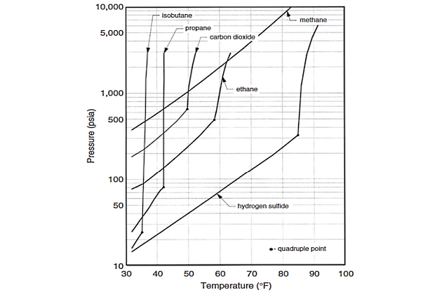
The extension to mixtures is not obvious from this diagram. The hydrate curve for multicomponent gaseous mixtures may be generated by a series of laboratory experiments or, more commonly, is predicted using thermodynamic software based on the composition of the hydrocarbon and aqueous phases in the system.
The thermodynamic understanding of hydrates indicates the conditions of temperature, pressure, and composition that hydrates are stable. However, it does not indicate when hydrates will form and, more importantly, whether they will cause blockages in the system.
Prediction of Hydrate Formation Conditions
There are numerous methods available for predicting hydrate formation conditions. Three popular methods for rapid estimation of hydrate formation conditions are discussed. A detailed discussion of other methods that are perhaps beyond the scope of the present discussion can be found in publications by Kumar, Sloan, and Carroll.
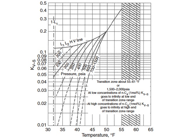
K-Factor Method. This method was developed originally by Carson and Katz, although additional data and charts have been reproduced since then. In this method, the hydrate temperature can be predicted using vapor-solid (hydrate) equilibrium constants. The basic equation for this prediction is:
where:
- y – is mole fraction of component i in gas on a water-free basis;
- Ki – is vapor-solid equilibrium constant for component i, and n is number of components.
The calculation is iterative, and the incipient solid formation point will determine when the aforementioned equation is satisfied. This procedure is akin to a dew point calculation for multicomponent gas mixture.
The vapor-solid equilibrium constant is determined experimentally and is defined as the ratio of the mole fraction of the hydrocarbon component in gas on a water-free basis to the mole fraction of the hydrocarbon component in the solid on a water-free basis:
where:
- xi – is mole fraction of component i in solid on a water-free basis.
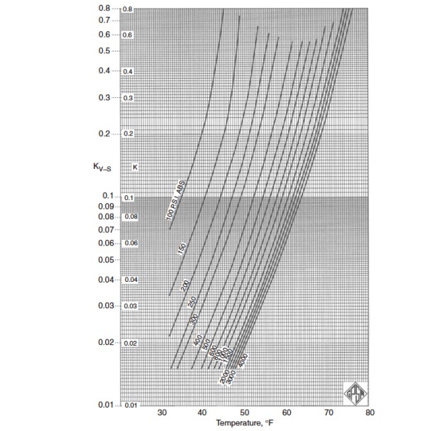
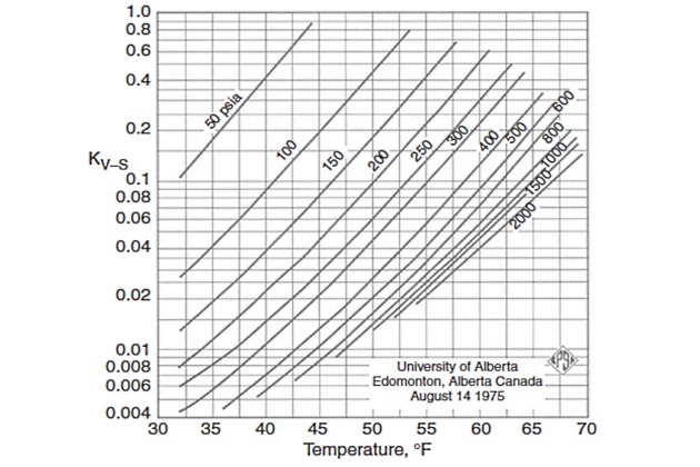
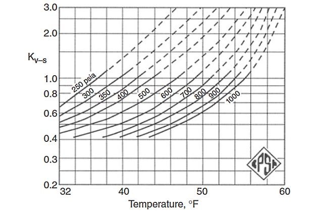
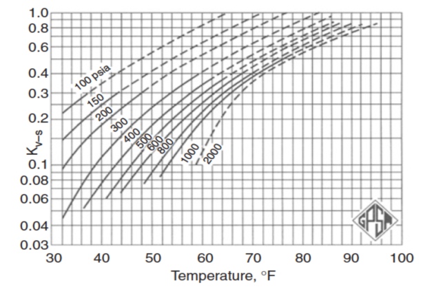
Figures 2 through 5 provide the vapor-solid equilibrium constants at various temperatures and pressures.
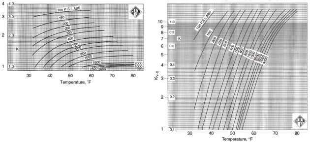
For nitrogen and components heavier than butane, the equilibrium constant is taken as infinity.
It should be stressed that in the original method of Carson and Katz it is assumed that nitrogen is a nonhydrate former and that n-butane, if present in mole fractions less than 5 %, has the same equilibrium constant as ethane. Theoretically, this assumption is not correct, but from a practical viewpoint, even using an equilibrium constant equal to infinity for both nitrogen and n-butane, provides acceptable engineering results.
The Carson and Katz method gives reasonable results for sweet Characteristics of Natural Liquefied Gasesnatural gases and has been proven to be appropriate up to about 1 000 psia.
However, Mann et al. presented new K-value charts that cover a wide range of pressures and temperatures. These charts can be an alternate to the Carson and Katz K-value charts, which are not a function of structure or composition.
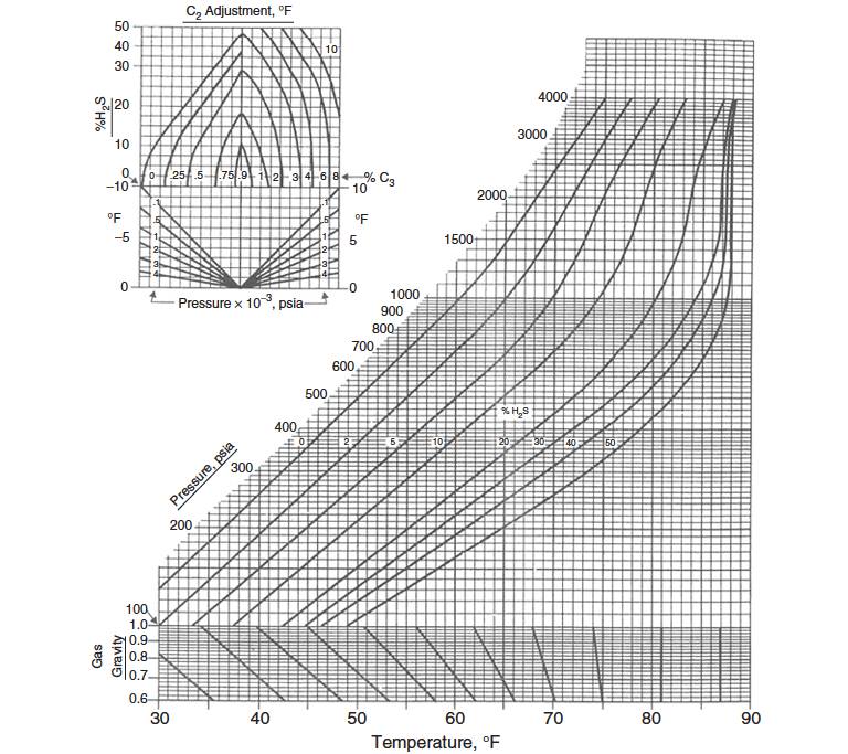
Baillie and Wichert Method. The method presented by Baillie and Wichert is a chart method (Figure 7) that permits estimation of hydrate formation temperatures at pressure in the range of 100 to 4 000 psia for natural gas containing up to 50 % hydrogen sulfide and up to 10 % propane. The method may not apply to a sweet gas mixture containing CO2, but is considered fairly accurate if the CO2 is less than about 5 mol%.
Gas Gravity Method. Until now, several other methods have been proposed for predicting hydrate-forming conditions in Usage of Equations of State in Liquefied Natural Gas Systems for Modeling Phase Behaviornatural gas systems. The most reliable of these requires a gas analysis.
However, if the gas composition is not known, even the previous methods cannot be used to predict the hydrate formation conditions, and the Katz gravity chart (Figure 8) can be used to predict the approximate pressure and temperature for hydrate formation, provided hydrates exist in the pressure-temperature region above the appropriate gravity curve.
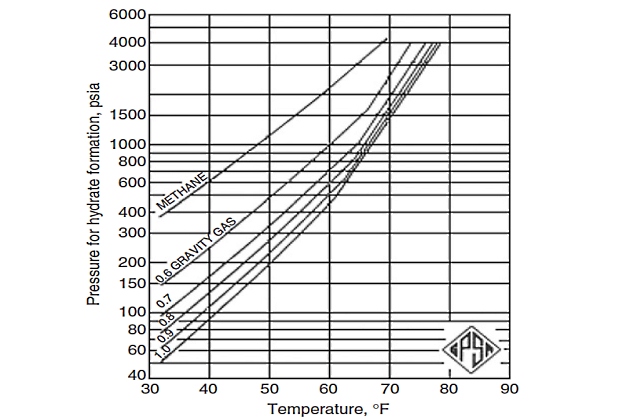
Therefore, as a first step to predict hydrate formation temperature, one can develop an appropriate equation representing the Katz gravity chart. Such a correlation uses two coefficients that correlate temperature, pressure, and specific gravity of gas:
where:
- T – is gas flow temperature, °F;
- P – is gas flow pressure, psia;
- and SG – is specific gravity of gas (air = 1,0).
Note that while Equation 4 is based on the GPSA chart, it is only accurate up to 65 °F. Beyond that it overestimates the temperature slightly.
The Katz gravity chart was generated from a limited amount of experimental data and a more substantial amount of calculations based on the K-value method. The components used for the construction of this chart are:
- methane,
- ethane,
- propane,
- butane,
- and normal pentane;
therefore, using this chart for compositions other than those used to derive these curves will produce erroneous results. In fact, this method is an appropriate method of estimating hydrate formation conditions for sweet natural gas mixtures. However, the Baillie and Wichert method is better than this chart when applied to sweet gas because of the inclusion of a correction factor for propane.
Commercial Software Programs. Hydrate formation conditions based on fluid compositions are normally predicted with the commercially available software programs. These programs are generally quite good and so simple to use that they often require less time than the simplified methods presented. The bases of these computer programs are the statistical thermodynamic models, which use a predictive algorithm with additional experimental data included to modify or “tune” the mathematical predictions. Most commercially available softwares use algorithms developed by D. B. Robinson and Associates (EQUIPHASE) and by Infochem Computer Services Ltd (MULTIFLASH). A detailed discussion of the accuracy of these programs and other hydrate software programs can be found in Sloan and Carroll.
Hydrate Prevention Techniques
As multiphase fluid flows through pipelines, it cools down, often reaching conditions where hydrates could form. Effective and economical prevention is necessary for normal pipeline operation.
Control relies on keeping system conditions outside the hydrate stability region, either by maintaining the fluid warmer than the hydrate formation temperature or by operating at a lower pressure.
While several methods exist, some onshore techniques (like line heaters and depressurization) are often impractical for long, high-pressure subsea pipelines.
For offshore transmission systems, the permanent, but often costly, solution is the removal of water using a large offshore dehydration plant. In general, the two main methods applicable at the well site are thermal and chemical techniques.
Thermal Methods. Thermal methods prevent hydrate formation by either conserving or introducing heat to keep the flowing mixture out of the hydrate formation range.
Heat conservation is common practice achieved through insulation. This method balances the high cost of insulation against system operability and acceptable risk, and is feasible for some subsea applications depending on fluid type and tieback distance.
To introduce heat, several concepts are available, including external hot-water jackets (in pipe-in-pipe or bundles) or conductive/inductive heat tracing. Electrical resistance heating is useful for long offset systems where insulation is insufficient, or during shut-in conditions.
It will be interesting: Conducting key ship operations – general information
Active heating systems offer environmentally friendly Cargo Temperature Control and Cargo Vent Systemstemperature control and increase production by avoiding time lost to depressurization, pigging, or blockage removal. However, operators remain hesitant to install these active heating systems.
Chemical Inhibition. An alternative to the thermal processes is chemical inhibition. Chemical inhibitors are injected at the wellhead and prevent hydrate formation by depressing the hydrate temperature below that of the pipeline operating temperature. Chemical injection systems for subsea lines have a rather high capital expenditure price tag associated with them, in addition to the often high operating cost of chemical treatment.
However, hydrate inhibition using chemical inhibitors is still the most widely used method for unprocessed gas streams, and the development of alternative, cost-effective, and environmentally acceptable hydrate inhibitors is a technological challenge for the Mastering Natural Gas Fundamentals Properties Sources and Transport Insightsgas production industry.
Types of Inhibitors. Traditionally, methanol, ethylene glycol (MEG), or triethylene glycol (TEG) are used as “thermodynamic inhibitors.” These high-concentration chemicals shift the hydrate stability curve, requiring a lower temperature or higher pressure for formation. Increasing salt content can also provide some suppression, though usually not enough alone.
Inhibitor selection involves comparing cost, safety, Chemical Composition and Physical Properties of Liquefied Gasesphysical properties, and, primarily, the feasibility of recovery and regeneration. Methanol is often preferred despite potential losses because its low viscosity and surface tension allow for effective separation at cryogenic conditions. Glycols, especially MEG, are frequently chosen due to their lower cost and reduced gas-phase losses, but they must be added at high rates (up to 100 % of water weight), necessitating expensive and large regeneration plants.
Because of the high cost of glycols, there is a need for low-dosage hydrate inhibitors (LDHIs). LDHIs offer substantial cost savings by requiring much lower concentrations and reducing the size of injection/storage facilities. Unlike thermodynamic inhibitors, LDHIs do not change the thermodynamic conditions; instead, they act at the early stages of formation by modifying the system’s rheological properties.
There are two types of LDHIs:
- “kinetic hydrate inhibitors” (KHIs),
- and “antiagglomerants” (AAs).
Most commercial kinetic inhibitors are high molecular weight polymeric chemicals (i. e., poly[N-vinyl pyrrolidone] or poly[vinylmethylacetamide/vinylcaprolactam]), which are effective at concentrations typically 10 to 100 times less than thermodynamic inhibitors concentrations. KHIs may prevent crystal nucleation or growth during a sufficient delay compared to the residence time in the pipeline.
Kinetic Hydrate Inhibitors (KHIs) delay hydrate formation. The deeper the system operates within the hydrate region, the shorter the achievable delay (ranging from weeks to hours). KHIs are relatively insensitive to the hydrocarbon phase, making them applicable to a wide range of systems. However, their industrial application depends on repeatable testing results across laboratory, pilot, and field settings.
In contrast, Anti-Agglomerants (AAs), which are surface-active chemicals, do not prevent crystal formation. Instead, AAs keep hydrate particles small and dispersed, maintaining low fluid viscosity so they can be transported with the produced fluids. AAs are effective at more extreme conditions than KHIs and their performance is relatively time-independent, making them attractive for deepwater fields (e. g., Gulf of Mexico, North Sea).
However, AAs have a major limitation: they require a continuous oil phase and are only applicable at low water cuts (typically 40-50 %).
Ultimately, the choice of inhibitor must be based on physical limitations and economics. Notably, unlike thermodynamic and kinetic inhibitors, the required dosage of an anti-agglomerant does not increase as the degree of subcooling increases, making AAs a potentially cost-effective solution under severe conditions.
Prediction of Inhibitor Requirements. The inhibitor must be present in a minimum concentration to avoid hydrate formation. Accurate prediction of this minimum inhibitor concentration is required for cost-effective design and operation of multiphase pipelines. Various empirical methods, charts, and computer programs have been developed for this purpose, including the venerable Hammerschmidt’s empirical equation, which is a relatively simple method that has been used to calculate the amount of inhibitor required in the water phase to lower the hydrate formation temperature:
where:
- ∆T – is depression of hydrate formation temperature, °F;
- MW – is molecular weight of inhibitor;
- W – is weight percentage of inhibitor in final water phase;
- and K – is constant, depending on the type of inhibitor.
Experimentally determined values of K and molecular weights of inhibitors are given in Table 2. To use this equation, the hydrate formation temperature in the gas without the inhibitor being present must be known. In fact, Equation 5 only predicts the deviation from the hydrate formation temperature without an inhibitor present.
| Table 2. Physical Constants of Inhibitors | ||
|---|---|---|
| Inhibitor | MW | K |
| Methanol | 32,04 | 2335 |
| Ethanol | 46,07 | 2335 |
| Isopropanol | 60,10 | 2335 |
| Ethylene glycol | 62,07 | 2200 |
| Propylene glycol | 76,10 | 3590 |
| Diethylene glycol | 106,10 | 4370 |
| Triethylene glycol | 150,17 | 5400 |
The Hammerschmidt equation is limited to inhibitor concentrations of about 20-25 wt % for methanol and 60-70 wt % for glycols.
However, for higher methanol concentrations, Nielsen and Bucklin have recommended the following equation:
where:
- XH2O – is the mole fraction of water in the aqueous phase.
They claim that this equation is accurate up to 90 wt % methanol, which gives the maximum suppression because methanol freezes at concentrations above 90 wt %. However, studies of GPSA only recommend the Nielsen and Bucklin equation for methanol concentrations ranging from 25 to 50 wt %. Equation 6 was developed for use with methanol; however, this equation is actually independent of the choice of inhibitor and therefore, theoretically, it can be used for any glycols.
Maddox et al. described a graphical procedure for estimating the required inhibitor concentration for both methanol and glycol. This method is a trial-and-error approach, which can be used when the activity coefficients of water in methanol and glycol are available. Although this method provides better accuracy, no recommended applicable range is provided.
If the produced water or seawater is in contact with the hydrocarbon fluid, the salinity of the water will itself inhibit hydrate formation. Therefore, it is important to be able to estimate the effect of the brine in the produced water on the hydrate formation temperature. For this purpose, McCain presented the following equation:
where:
- ∆T – is temperature depression, °F;
- and S – is water salinity, wt %.
Equation 7 is limited to salt concentrations of less than 20 wt % and for gas-specific gravities (SG) ranging from 0,55 to 0,68.
All of these simple methods predict the depression of the hydrate formation temperature; they do not predict the actual hydrate formation conditions. However, several thermodynamic models have been proposed for predicting the hydrate formation conditions in aqueous solutions containing methanol/glycols and electrolytes. These rigorous models can also account for the effect of pressure and the type of hydrate neglected in the simple mentioned methods. However, available models have limitations that include the types of liquid, compositions of fluids, and inhibitors used.
The amount of inhibitor required to treat the water phase, plus the amount of inhibitor lost to the vapor phase and the amount that is a soluble in the hydrocarbon liquid, equals the total amount required. Methanol vaporization loss can be estimated from Figure 9, while glycol vaporization losses are generally very small and typically can be ignored.
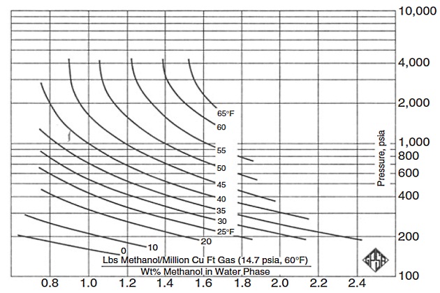
In addition, prediction of inhibitor losses to the hydrocarbon liquid phase is difficult. However, many of the commercially available software programs include proper calculations to account for the loss of methanol and glycols to the hydrocarbon liquid phase.
Design of Injection Systems. Proper design of an inhibitor M-type electronically controlled gas injection (ME-GI)injection system is complex, requiring optimum inhibitor selection, determination of injection rates, pump sizing, and pipeline diameters.
Selecting inhibitors for a subsea gas transmission system is difficult because key factors affecting performance (like brine composition, temperature, and pressure) are unknown before production starts. Therefore, designers must use appropriate multiphase flow simulation packages to calculate necessary unknown variables.
To determine the appropriate injection rate, field testing is preferable. These requirements dictate the necessary storage, pumping capacity, and number of lines to ensure delivery during start-up and shut-in.
Read also: Planning the Design, Construction and Operation of New LNG Transportation Systems
Injection points should be chosen for maximum benefit, generally at the center of the pipe in the flow direction. However, the exact rate and location depend on flow geometry, fluid properties, and P-T relationships encountered in the field.
For deepwater systems, inhibitors are often pumped through long, small-diameter umbilicals. The injection pump is a positive displacement metering pump capable of generating high pressure (typically 3 000 – 4 000 psi) to overcome the line operating pressure. Ideally, the injection pressure should be 100 psi above the line pressure, and varied rates are achieved by changing this differential pressure. Ramachandran et al. discuss the proper design and behavior prediction of deepwater injection systems.
Corrosion
One of the common problems in multiphase flow transmission pipelines is metal corrosion. Corrosion is defined as the deterioration of material, usually a metal, due to its reaction with the environment or handling media. The cause of corrosion can be directly attributed to the impurities found in the produced gas, as well as the corrosive components that are by-produced. Because of the nonspecificity of the components produced from a production well, some or all of these components may be active to create a corrosive environment in the pipelines. Corrosion in multiphase systems is a complex phenomenon, including dependency on the partial pressure, temperature, pH, and concentration of corrosion products.
Consequently, corrosion prediction requires substantial understanding of the simultaneous interaction of the many process variables that govern both flow and corrosion conditions.
An important aspect of maintaining pipeline performance is adequate control of corrosion both internally-caused by the flow components and their by-products – and externally – because of pipeline exposure to the soil and water. Pipeline corrosion can be inhibited by several means.
- Choice of corrosion-resistant metals, alloys.
- Injection of corrosion inhibitors.
- Сathodic protection.
- External and/or internal protective coatings.
While corrosion control can be achieved by selection of an appropriate corrosion-resistant metal, operating considerations usually dictate that a high-efficiency corrosion control system be used. Protecting pipelines from corrosion is achieved internally by the injection of inhibitors to mitigate internal corrosion and externally by use of cathodic protection and/or a combination of coatings and cathodic protection (for buried or subsea pipelines).
Choice of Corrosion-Resistant Metals
Corrosion resistance is a basic property related to the ease with which materials react with a given environment. All metals have a tendency to return to stable conditions. This tendency causes metals to be classified according to rising nobleness, which again leads to classification of decreasing activity and increasing potential. For specific recommendations concerning materials selection, refer to the ANSI B31.3 and B31.8, API RP 14E and NACE MR-01-75. Corrosion resistance is not the only property to be considered in the material selection process, and the final selection will generally be the result of several compromises between corrosion resistance and economic factors.
Historically, high-strength steels and alloys Corrosion-resistant alloys, such as 13 % Cr steel and duplex stainless steel, are often used downhole and, recently, for short flow lines; however, for long-distance, large-diameter pipelines, carbon steel is the only economically feasible material.x have been the safest and most economical materials for the construction of offshore transmission pipelines. However, the inherent lack of corrosion resistance of these materials in subsea pipelines requires a corrosion control system with a high degree of reliability.
Corrosion Inhibitors
Chemical corrosion inhibitors are cationic surfactants used in small concentrations to effectively reduce the metal corrosion rate. These inhibitors, typically organic chemicals containing nitrogen (amines) in petroleum applications, adsorb onto the metallic surface to form a corrosion-resistant film. A key advantage is their ability to respond to increases in the corrosive environment.
Inhibitors can be applied in batches to create a long-lasting protective film, or continuously injected in low concentrations to maintain a thin film. A combination of periodic large batches followed by continuous low-concentration treatment is also used.
While traditional studies relied on laboratory results, recent efforts focus on developing environmentally friendly approaches for corrosion control in multiphase pipelines. One such technique involves increasing the water phase pH using agents like sodium hydroxide to facilitate the formation of a dense iron carbonate film. However, these carbonate films are often not stable under slugging conditions and are unsuitable for brines with high chloride concentrations.
Cathodic Protection
Cathodic protection is the most successful method for reducing or eliminating corrosion for buried or submerged metallic structures that involves using electric voltage to prevent corrosion.
When two metals are connected to each other electrically in an electrolyte (e. g., seawater), electrons will flow from the more active metal (anode) to the other (cathode) due to the difference in the electrochemical potential. The anode supplies current, and it will gradually dissolve into ions in the electrolyte and at same time produce electrons that the cathode will receive through the metallic connection with the anode. The result is that the cathode will be negatively polarized and hence be protected against corrosion. The two methods of achieving cathodic protection are:
- the use of sacrificial or reactive anodes with a corrosion potential lower than the metal to be protected;
- and applying a direct current.
Use of a direct current system is less costly than sacrificial anodes and provides a higher range of possible potential differences, although they may require greater maintenance during the lifetime of the operation.
Protective Coatings
While cathodic protection has historically been employed as the sole corrosion control methodology for subsea gas production systems, the nature of multiphase pipelines is such that the combined use of protective coatings with cathodic protection is necessary to achieve the effective protection For some installations (e. g., deepwater) one might choose continuous inhibition over protective coating due to the implications of a coating failure.x. In fact, protective coatings help control pipeline corrosion by providing a barrier against reactants such as oxygen and water. However, because all organic coatings are semipermeable to oxygen and water, coatings alone cannot prevent corrosion and so a combination of cathodic protection is often used.
Pipelines use internal coatings like epoxies or plastics primarily to minimize corrosion before construction and to provide a smooth surface that reduces fluid friction during transit. It’s often most economical to protect pipelines early in a field’s life due to high initial corrosiveness. The coating must be compatible with the commodity and resistant to contaminants.
External coatings are essential for reducing external corrosion by creating a high electrical resistance barrier between the metal and the environment, using materials like polyurethane or fusion-bonded epoxy.
Since pipelines are susceptible to both internal and external corrosion, comprehensive monitoring is required. While traditional inspection methods assess pipeline condition, the newer Field Signature Method (FSM) offers a more sensitive and accurate solution. FSM continuously monitors corrosion and pipe wall thickness at a specific point, immediately transferring data to the surface. This technique reduces costs, improves safety, and may decrease the need for frequent intelligent pigging, with a service life equal to the pipe itself, though it is still a relatively new technology.
Wax
Multiphase flow can be severely affected by the deposition of organic solids, usually in the form of wax crystals, and their potential to disrupt production due to deposition in the production/transmission systems. The wax crystals reduce the effective cross-sectional area of the pipe and increase the pipeline roughness, which results in an increase in pressure drop. The deposits also cause subsurface and surface equipment plugging and malfunction, especially when oil mixtures are transported across Arctic regions or through cold oceans. Wax deposition leads to more frequent and risky pigging requirements in pipelines. If the wax deposits get too thick, they often reduce the capacity of the pipeline and cause the pigs to get stuck. Wax deposition in well tubings and process equipment may lead to more frequent shutdowns and operational problems.
Wax Deposition
Precipitation of wax from petroleum fluids is considered to be a thermodynamic molecular saturation phenomenon. Paraffin wax molecules are initially dissolved in a chaotic molecular state in the fluid. At some thermodynamic state the fluid becomes saturated with the wax molecules, which then begin to precipitate. This thermodynamic state is called the onset of wax precipitation or solidification. It is analogous to the usual dew point or condensation phenomenon, except that in wax precipitation a solid is precipitating from a liquid, whereas in condensation a liquid is precipitating from a vapor. In wax precipitation, resin and asphaltene micelles behave like heavy molecules. When their kinetic energy is sufficiently reduced due to cooling, they precipitate out of solution but they are not destroyed. If kinetic energy in the form of heat is supplied to the system, these micelles will desegregate and go back into stable suspension and Brownian motion.
Wax Deposition Envelope. Many reservoir fluids at some frequently encountered field conditions precipitate field waxes. It is very important to differentiate field waxes from paraffin waxes. Field waxes usually consist of a mixture of heavy hydrocarbons such as:
- asphaltenes,
- resins,
- paraffins (or paraffin waxes),
- cyclo-paraffins,
- and heavy aromatics.
Wax precipitation depends primarily on fluid temperature and composition and is dominated by van der Waals or London dispersion type of molecular interactions. Pressure has a smaller effect on wax precipitation. As with asphaltenes, the fact that waxes precipitate at some and not at other thermodynamic states, for a given fluid, indicates that there is a portion of the thermodynamic space that is enclosed by some boundary within which waxes precipitate. This bounded thermodynamic space has been given the name wax deposition envelope (WDE).
A typical WDE is shown in Figure 10.
The Wax Disappearance Envelope (WDE) boundary is an important characteristic of reservoir fluids. The upper WDE boundary is often observed as nearly vertical when measured experimentally. The intersection of the WDE boundary with the bubble-point line is typically to the left of the stock tank oil’s cloud point (onset of wax crystallization). This is because light ends suppress the wax crystallization temperature when pressured into the oil. The lower WDE boundary’s shape depends mainly on the composition of the fluid’s intermediates and light ends.
Measuring the complete WDE is often not economical due to the relatively new and expensive technology. Therefore, companies prefer to obtain only a few experimental data points to fine-tune phase behavior models. Currently, most of these models lack strong predictive capacity and are primarily used as correlational-predictive tools, often due to improper or inadequate crude oil characterization.
It will be interesting: The role of the government in ensuring the development of the gas sector, key factors and principles
Gas/Condensate. Wax Deposition Envelope Some gas/condensates, especially rich gas/condensates with yields in excess of 50 bbls/MMSCF, are known to contain high carbon number paraffins that sometimes crystallize and deposit in the production facilities. The obvious question is what is the shape of the thermodynamic envelope (i. e., P and T surface) of these gas/condensates within which waxes crystallize or, in order to maintain the previous terminology, what is the WDE of gas/condensates typically?
The shapes of the WDEs of two gas/condensates in the Gulf of Mexico are presented here. The shapes of the aforementioned WDEs indicate potential wax deposition in those cases where the gas/condensate contains very high carbon number paraffins that precipitate in solid state at reservoir temperature. In other words, the temperature of the reservoir may not be high enough to keep the precipitating waxes in liquid state. Hence, the gas/condensate, which is a supercritical fluid, enters the WDE at the “dew point” pressure. This casts new insight into the conventional explanation that the productivity loss in gas/condensate reservoirs, when the pressure near the wellbore reaches the dew point, is only due to relative permeability effects.
Figure 11 shows the vapor-liquid (V-L) envelope of what one might call a typical Gulf of Mexico gas/condensate. This gas/condensate (called gas/condensate “A” for our purposes here) was analyzed with PARA (paraffin-aromatic-resin-asphaltene) analysis and found to contain normal paraffins with carbon numbers exceeding 45.
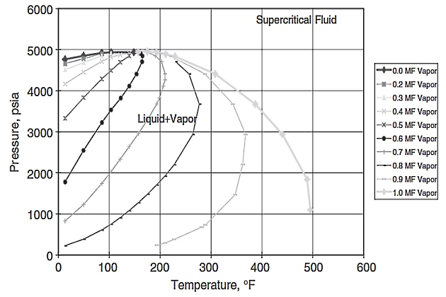
The V-L envelope was simulated using the Peng and Robinson original equation of state (EOS) that had been fine-tuned to PVT data obtained in a standard gas/condensate PVT study. The first question that was addressed in a wax study involving this fluid was what happens as the fluid is cooled at some constant supercritical pressure? What actually happened is shown in Figure 12.
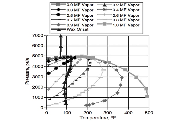
Figure 12 shows several onset of wax crystallization data points obtained with near-infrared (NIR) equipment by cooling the gascondensate “A” at different constant pressures. It was evident from NIR data that there was a thermodynamic envelope, similar to the one defined and obtained experimentally for oils, to the left of which (i. e., at lower temperatures) wax crystallization occurred. The complete wax deposition envelope shown in Figure 12 was calculated with a previously tuned wax phase behavior model.
Despite the clarity of the WDE obtained for gas/condensate “A” as shown in Figure 12, more data were needed to confirm the presence of WDE in other condensates and establish its existence as a standard thermodynamic diagram.
Figure 13 shows the V-L envelope of another typical Gulf of Mexico condensate. This condensate (called gas/condensate “B” for our purposes here) also contains paraffins with carbon numbers exceeding 45, although data show that gas/condensate “B” is lighter than gas/condensate “A“. The V-L envelope was again simulated using the Peng and Robinson original EOS after it had been tuned to PVT data obtained in a standard gas/condensate PVT study.
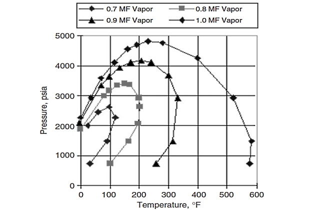
Figure 14 shows NIR onset data superimposed on the V-L envelope.
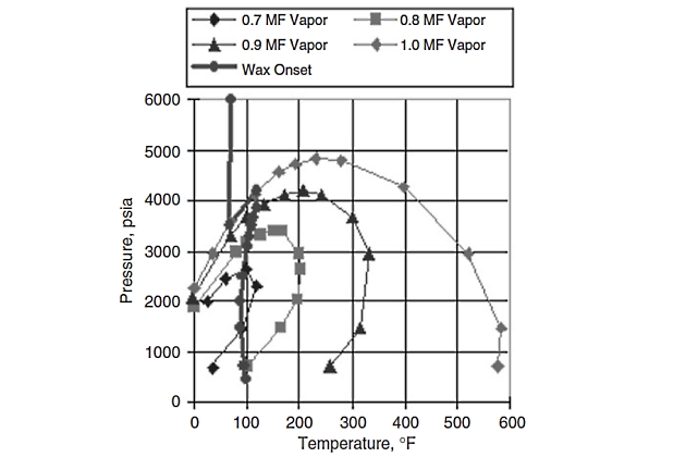
It is evident again from NIR data that there is a thermodynamic envelope to the left of which (i. e., at lower temperatures) wax crystallization occurs. Once again, the complete wax deposition envelope shown in Figure 14 was calculated with a previously tuned wax phase behavior model.
The data confirms the existence of a Wax Disappearance Envelope (WDE) in gas condensates containing paraffins of carbon number ≥45. This WDE is similar to those found in oils and should be considered a standard thermodynamic diagram.
Inside the vapor-liquid (V-L) envelope, the WDE initially shows a negative slope (tilts left) as pressure rises. This is due to light hydrocarbons suppressing wax crystallization. However, once retrograde condensation begins, the WDE turns forward, acquiring a positive slope. This shift occurs because light ends vaporize, increasing the concentration of waxes in the remaining liquid phase.
In most condensates, the WDE appears to coincide with the V-L saturation line until the temperature is low enough for wax crystallization to begin from the supercritical condensate. This behavior aligns with prior observations that supercritical hydrocarbon fluids (like propane or CO2) have increased solvent power, meaning they require cooling to much lower temperatures before paraffin waxes start to crystallize.
Wax Formation in Multiphase Gas/Condensate Pipelines
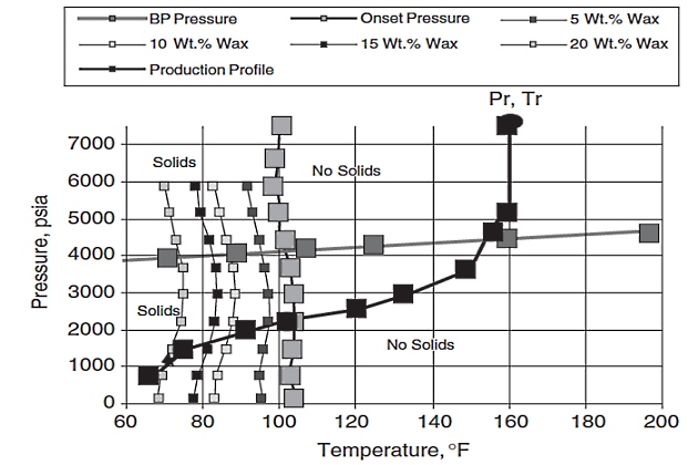
When the production pressure and temperature profile of a gas/condensate crosses the WDE and the hydrate envelope (HE), waxes and hydrates may form. The formed hydrates can grow in mass and yield strength to the point that they restrict and finally stop the flow. If the waxes form while the liquid is in contact with the wall, some of them should attach to the wall, thus resulting in wax deposition. Figure 15 shows a P-T diagram of a Gulf of Mexico gas/condensate demonstrating this situation.
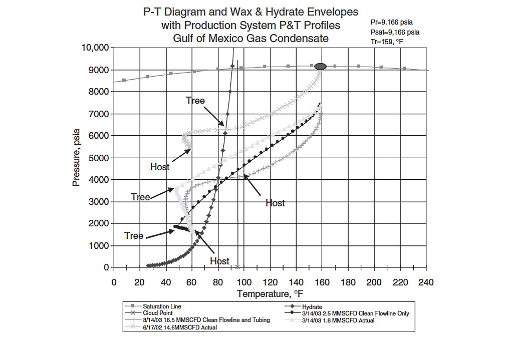
The diagram indicates that there was not any live NIR done with this fluid. The only point on the WDE that was measured was the cloud point of the condensate, shown in Figure 15 at 95 °F at the bottom of the vertical line. The clean tubing and flow line of this system would deliver about 14,5 MMSCFD on 6/17/2002. From the light blue P and T profile line and dark blue hydrate line, it was very clear at the outset that the main flow assurance issues in this system would be hydrate and wax formation and deposition. Hence, because of this illustrative important information, the effort to obtain the aforementioned diagram is obviously very worthwhile.
Read also: Wave and Impact Loads in Design of Large and Conventional Liquefied Gas Carriers
Sometimes oil and gas operators decide to design the facilities such that their operation is to the left of the WDE and HE (such as the example in Figure 15). In these situations, wax and hydrate formation takes place if the fluids are left untreated with chemicals. In the aforementioned example, methanol was injected to inhibit successfully the formation of hydrates formed due to the production of reservoir equilibrium water. However, because the operator was not aware of the wax phase behavior of this condensate at start-up, no wax chemical was injected. Wax deposition was severe enough to cause the production rate to drop to 1,8 MMSCFD on 3/14/2003. The estimated via simulation maximum production rate on 3/14/2003 was 16,5 MMSCFD. Data in the plot show that the maximum friction loss was in the upper part of the tubing.
Identification of Wax Deposition Problems. A rather simple chart that allows daily monitoring of wax deposition problems in multiphase gas/condensate pipelines is shown in Figure 16.
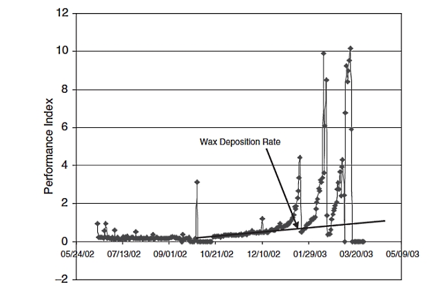
This chart is for the gas/condensate shown in Figure 15. The chart was made by plotting the performance index (PI) versus time. The PI is calculated from the following equation:
where:
- ∆P – is the pressure drop in the pipeline, psi‘
- and Q – is the flow rate, MMSCFD.
The PI should remain as a horizontal straight line during production if there is no restriction formed in the line. It is evident in Figure 16 that around 10/21/2002 a restriction was being formed in the line. At the beginning of January there was a very sharp loss of hydraulic capacity.
This cannot be due to wax deposition because the rate of wax deposition does not change so sharply in a produced fluid. Indeed, the sharp rise in the PI was caused by hydrate formation that occurred on top of wax crystal formation and deposition. Several sharp rises in PI followed caused by hydrates until it was determined that the well started producing free water and required a much higher methanol injection rate.
While all of this is happening with the advent of water and hydrate formation the wax deposition rate was increasing steadily, as shown on the chart.
It should be noted that the engineer needs to be very careful in attributing a rise in the PI only to wax and hydrates. One needs to make sure that other culprits, such as fines, salts, returning drilling, and completion fluids, are not present.
Wax Deposition Inhibition/Prevention. Engineers face challenges determining the wax deposition mechanism and effective chemical treatment in gas/condensate systems. In oil flow lines, wax deposits via diffusion and attachment to the wall. Inhibition involves injecting chemicals above the cloud point to modify wax crystals, reducing their attraction to the wall so they can be removed by fluid shear.
However, this classic mechanism (crystal forming at the wall) is typical for liquid-filled, uninsulated lines with fast heat transfer and diffusion. This is often not the case in gas/condensate flow lines. Here, the gas cools quickly in the main flow, forming wax crystals that tend to deposit or settle by gravity in the liquid holdup. Furthermore, these lines are often treated with methanol to prevent hydrates. Since most wax inhibitors are incompatible with alcohols/glycols, the inhibited wax crystals accumulate in the liquid holdup, forming a highly viscous, but movable, material called “wax slush“.
Field data and simulations support this “wax slush” theory. Direct evidence emerged during a hurricane-related shutdown: a fast well restart, intended to induce a slug and mobilize the slush, successfully did so. The mobilized wax slush flowed into separators, plugging lines and equipment and temporarily disabling operations.
It is appropriate at this time to give a brief description of the main two chemical classes used to treat wax deposition. There are three types of wax crystals:
- Plate crystals.
- Needle crystals.
- Mal or amorphous crystals.
Paraffinic oils form plate or needle crystals. Asphaltenic oils form primarily mal or amorphous crystals. Asphaltenes act as nucleation sites for wax crystal growth into mal crystals.
Plate crystals look as their name implies, like plates under the microscope. Needle crystals look like needles, and mal crystals are amorphous and generally look like small round spheres. The interaction between crystals and pipe wall increases from mal to needle to plates. Thus, maintaining newly formed wax crystals small and round, i. e., like mal crystals, is desirable.
The behavior and properties, e. g., cloud point and pour point, of paraffin crystals precipitating from a hydrocarbon can be affected in three ways.
- Crystal size modification: modification of the crystal from larger sizes to smaller sizes.
- Nucleation inhibition: inhibition of the growth rate of the crystal and its ultimate size.
- Crystal type or structure modification: modification of the crystal from one type to the other. For instance, modify a crystal from needle to mal type.
Wax crystal modifiers (also called pour point depressants or PPDs) primarily modify the size of wax crystals. By interrupting the normal growth of n-paraffins, they result in much smaller crystals. These smaller crystals have lower molecular weights, higher solubility in oil, and reduced interaction energy with each other and the pipe wall, effectively suppressing the crude oil’s pour point.
A wax dispersant works differently: it may inhibit wax nucleation and change the crystal structure from plate/needle to amorphous. Amorphous crystals are smaller and easier for the flowing fluid to carry. The presence of asphaltenes and resins enhances the dispersant’s effect, as the dispersant interacts with and removes these components, which act as nucleation sites for wax growth. When added above the cloud point, a dispersant can sometimes also suppress the cloud point. Dispersants also tend to disperse wax particles at the water-oil interface.
It will be interesting: Basic Knowledge of Tankers
Both modifiers and dispersants diminish wax formation and deposition through different mechanisms. Dispersants are generally smaller in molecular weight than modifiers, giving them more favorable viscosity and flow properties for cold applications. Some dispersants are also compatible with alcohols and glycols, allowing for simultaneous injection. Chemical selection should always be based on the specific hydrocarbon and facility characteristics.
Wax Deposit Remediation. On occasion, if a substantial amount of wax accumulates in the line, as evidenced by the PI chart such as the one shown in Figure 16, a temporary shutdown to do a chemical soak, with a potential modification to the chemical to give it more penetrating power at cold temperatures, and a fast start-up might be necessary to cause the wax slush cough.
Pigging is an option, but only after very careful consideration of the system’s performance to understand the dynamics of the moving pig and continuous removal of the wax cuttings ahead of it. This is a very difficult job. Controlling the bypass of flow around the pig for such a purpose is difficult. Hence, many pigging operations end up in failure with stuck pigs.
The pigging analysis and decision must be left to true experts. Starting a pigging program at the beginning of the life of the system has a better chance of success than at any other time. Even then, excellent monitoring of the system’s PI is a must. It is recommended that a short shutdown, chemical soak, and fast start-up be considered first, because it is the safest option.
Controlled Production of Wax Deposits. From a technical stand-point, spending enough capital initially to design the facilities to operate outside the wax and hydrate forming conditions or to the right of the WDE and HE is obviously the best solution. However, very often in practice, controlling wax deposits during production is preferred because of the lower facilities cost. Economically marginal fields can only be produced under this scenario. Hence, in these cases, the following three options prevail.
- Pigging only.
- Chemical injection only.
- Combination of pigging and chemical injection.
While frequent pigging of the line clears up any wax deposits, it may be necessary to chemically inhibit wax deposition during times when pigging is unavailable. Pigging often is inadequate or uneconomical unless used in conjunction with a chemical treatment program. This program is often performed into two stages:
- removal of wax deposits in the production/transmission lines;
- and continuous chemical injection or periodic treatment (such as batch treatments, etc.) in order to ensure pipeline integrity.
Chemical injection is the safest of the three if good technical support and testing are available. The approach is discussed as follows.
- Inject a strong chemical dispersant/inhibitor down the hole to keep the formed wax particles small and suspended in the flow line. The majority of them would be carried away with the gas/liquid flow.
- The chemical dispersant/inhibitor must be compatible and soluble with methanol to prevent precipitation of the chemical itself in the line.
- Monitor the hydraulics in the flow line and occasionally, if necessary, cause a “slug” or “cough” to cough up any accumulated wax.
- On occasion, if a substantial amount of wax accumulates in the line, a temporary shutdown to do a chemical soak, with a modification to the chemical to give it more penetrating power at cold temperatures, and a fast start-up might be necessary to cause the wax slush cough.
Severe Slugging
One of the most complex multiphase flow patterns with unsteady characteristics is intermittent or slug flow. Slug flow exists in the whole range of pipe inclinations and over a wide range of fluid flow rates.
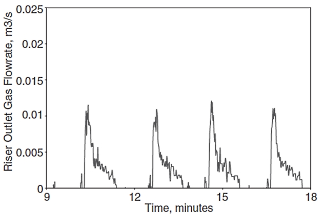
However, liquid slugs may, depending on the pipeline geometry and flow conditions, become very large (severe slugging) and threaten the safe and reliable operation of a production system. Severe slugging can occur in a multiphase flow system, operating at low liquid and gas flow rate, where a downward inclined pipe segment is followed by an upward inclined segment/riser. For this system, liquid will accumulate in the riser and the pipeline, blocking the flow passage for gas flow. This results in a compression and pressure buildup in the gas phase that will eventually push the liquid slug up the riser and a large liquid volume will be produced into the separator that might cause possible overflow and shut down of the separator. The severe slugging phenomenon is very undesirable due to pressure and flow rate fluctuations, resulting in unwanted flaring and reducing the operating capacity of the separation and compression units. Figures 17 and 18 show example time traces for the riser outlet liquid and gas flow rates during severe slugging, respectively.
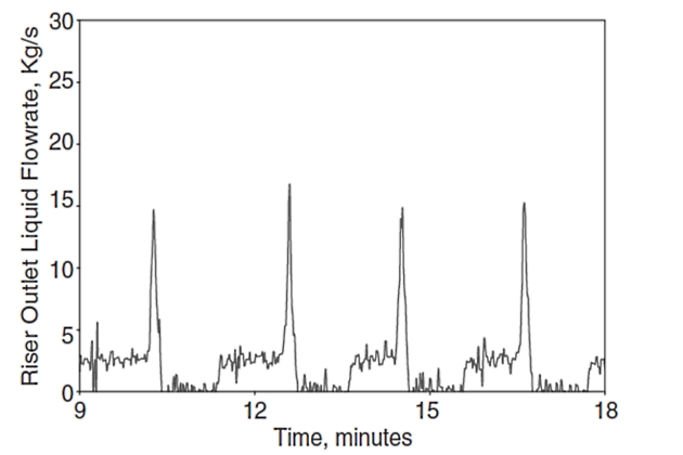
These figures show the large surges in liquid and gas flow rates accompanying the severe slugging phenomenon. Clearly such large transient variations could present difficulties for topside facilities unless they are designed to accommodate them.
Operators typically avoid operating in the severe slugging region, but inlet conditions of production pipelines are influenced by factors like well capacity and operational events (shutdowns/restarts).
In offshore production, overdimensioning separators to avoid critical flooding is often too costly or impossible. Design engineers therefore require more accurate dynamic simulations and high-performance control systems to manage production schemes that are highly sensitive to transients caused by slug flow. Achieving correct simulation results, especially for severe slugging dynamics, requires a tight integration of the hydrodynamic model (pipeline-riser system) with the dynamic model of the receiving plant.
Understanding the formation, prevention, and control of severe slugging is crucial. Although there is research on severe slugging in flexible risers, a lack of widely available transient code testing and full-scale data prevents better understanding of the physics and limits rigorous verification. This deficit in real-world validation hinders the confidence of designers and operators in expanding the use of flexible risers in critical applications.
Severe Slugging Mechanism
The process of severe slugging in a pipeline-riser system consists of four steps:
- slug formation,
- slug production,
- bubble penetration,
- and gas blow down.
This phenomenon had been identified previously by Schmidt et al. as a cyclic flow rate variation, resulting in periods of both no flow and very high flow rates substantially greater than the time average. Figure 19 illustrates the stages of a severe slugging cycle.
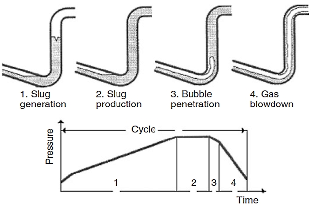
The severe slugging process in a riser is a four-step cycle:
- Slug Formation: Pipeline pressure builds up until the liquid level in the riser reaches the top. Gas is no longer supporting the liquid, which falls and blocks the riser entrance.
- Slug Production: The liquid slug is produced until gas reaches the riser base.
- Bubble Penetration: Gas enters the riser, decreasing hydrostatic pressure and increasing gas flow.
- Gas Blow Down: Gas reaches the top, pressure is minimal, and the liquid level falls, starting a new cycle.
This cycle is steady state if gas penetration into the riser remains positive. Alternatively, if gas penetration drops to zero, liquid blocks the riser base, causing the liquid interface to move into the pipeline until it retreats, and a new cycle begins.
Depending on the liquid input, two types of cyclic processes occur: without fallback (liquid fills the riser completely) or with fallback (low liquid input causes gas accumulation at the top as liquid falls back). Essentially, three different scenarios can result from gas penetrating a liquid column during severe slugging.
- Penetration of the gas that leads to oscillation, ending in a stable steady-state flow.
- Penetration of the gas that leads to a cyclic operation without fallback of liquid.
- Penetration of the gas that leads to a cyclic operation with fallback of liquid.
Severe slugging in a pipeline-riser system can be considered a special case of flow in low-velocity hilly terrain pipelines, which are often encountered in an offshore field. This is a simple case of only one downward inclined section (pipeline), one riser, and constant separator pressure. For this reason, severe slugging has been termed “terrain-induced slugging“. This phenomenon has also various names in the industry, including “riser-base slugging” and “riser-induced slugging“.
Stability Analysis
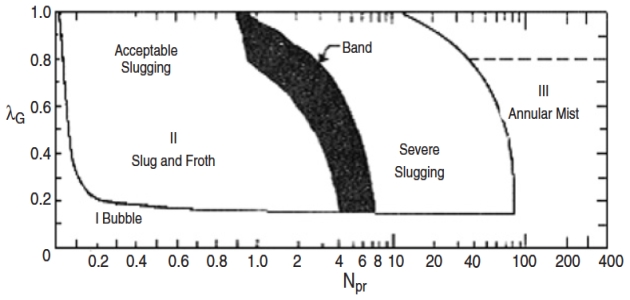
The flow characteristics of multiphase flow in a pipeline-riser system are divided into two main regions: stable (steady flow) and unstable (pressure cycling), in which the stability line on the flow pattern map separates the two regions. The steady region includes acceptable slugging, annular mist, and bubble flows, whereas the pressure cycling region includes severe slugging and transitional flows. Figure 18 shows a typical flow map for a pipeline-riser system developed by Griffith and Wallis featuring regions of stable and unstable behavior.
In Figure 20, NFr and λG are the Froude number of two-phase gas/liquid flow and no-slip gas holdup, defined previously. As it can be seen from Figure 18, at low Froude numbers, bubble flow prevails and fluids will flow through riser pipes without slug formation. However, as the Froude number increases, the slug flow range is entered.
The stability analysis predicts the boundary between stable and unstable regions, where the resultant stability map helps the engineer to design systems that operate well into the stable zone, thus offering an adequate margin of safety. The stability analysis seeks to model a particular process required for severe slugging and hence predicts the likelihood of severe slugging, as such these stability models are termed criteria for severe slugging. The severe slugging process was first modeled by Schmidt et al.; however, their model formed the basis of much of the early work for the stability of severe slugging. A review of the existing stability criteria for predicting severe slugging in a pipeline-riser system can be found in Mokhatab.
Prevention and Control of Severe Slugging
The flow and pressure oscillations due to severe slugging phenomenon have several undesirable effects on downstream topside facilities unless they are designed to accommodate them. However, designing topside facilities to accept these transients may dictate large and expensive slug catchers with compression systems equipped with fast-responding control systems. This may not be cost-effective and it may be more prudent to design the system to operate in a stable manner. While lowering production rates (slowing fluid velocity) can minimize severe slugging, operators are investigating alternatives that would allow for maximum production rates without the interruptions caused by slugs.
Mokhatab et al. reference a combination of industrial experience and information from the literature to compile a list of methods of remediating the problems associated with severe slugging in pipeline-riser systems. In general, severe slugging prevention and elimination strategies seek the three following approaches.
Read also: Overview of the Carriage of Liquefied Gases by Sea
Riser Base Gas Injection. Riser base gas injection is a frequently used method that provides artificial lift and can mitigate hydrodynamic slugging by changing the flow regime (from slug to annular/dispersed). However, it is ineffective against transient slugging and can cause issues in deepwater systems due to high frictional pressure loss and Joule-Thomson cooling. Early studies questioned its economic feasibility due to compression and piping costs, though later work confirmed it significantly reduces slugging severity.
The potential for Joule-Thomson cooling to induce wax precipitation and hydrate formation led to alternatives. Johal et al. proposed “multiphase riser base lift“, diverting nearby high-capacity multiphase lines to alleviate slugging without exposing the system to cooling issues.
More recently, Sarica and Tengesdal proposed a “self-gas lifting” technique. This method uses a small-diameter conduit to connect the riser to the downward inclined pipeline segment, transferring gas to points above the riser base (multiposition gas injection). This reduces the hydrostatic head in the riser and pipeline pressure, which lessens or eliminates severe slugging. This low-cost method is expected to increase production by avoiding additional backpressure on the system.
Topside Choking. This method induces bubble flow or normal slug flow in the riser by increasing the effective backpressure at the riser outlet. While a topside choke can keep liquids from overwhelming the system, it cannot provide required control of the gas surges that might be difficult for the downstream system to manage. This is a low-cost, slug mitigation option, but its application might be associated with considerable production deferment.
Topside chocking was one of the first methods proposed for control of the severe slugging phenomenon. Yocum observed that increased backpressure could eliminate severe slugging but would reduce the flow capacity severely. Contrary to Yocum’s claim, Schmidt et al. noted that the severe slugging in a pipeline-riser system could be eliminated or minimized by choking at the riser top, causing little or no changes in flow rates and pipeline pressure. Taitel provided a theoretical explanation for the success of choking to stabilize the flow as described by Schmidt et al.
Jansen investigated different elimination methods, such as gas-lifting, chocking, and gas-lifting and chocking combination. He proposed the stability and the quasi-equilibrium models for the analysis of the aforementioned elimination methods. He experimentally made three observations:
- large amounts of injected gas were needed to stabilize the flow with the gas-lifting technique;
- careful chocking was needed to stabilize the flow with minimal backpressure increase;
- and the gas-lifting and chocking combination were the best elimination method, reducing the amount of injected gas and the degree of choking to stabilize the flow.
Control Methods. Control methods (feedforward control, slug choking, active feedback control) for slug handling are characterized by the use of process and/or pipeline information to adjust available degrees of freedom (pipeline chokes, pressure, and levels) to reduce or eliminate the effect of slugs in the downstream separation and compression unit. Control-based strategies are designed based on simulations using rigorous multiphase simulators, process knowledge, and iterative procedures. To design efficient control systems, it is therefore advantageous to have an accurate model of the process.
The feedforwarded control aims to detect the buildup of slugs and, accordingly, prepares the separators to receive them, e. g., via feedfor-warded control to the separator level and pressure control loops. The aim of slug choking is to avoid overloading the process facilities with liquid or gas. This method makes use of a topside pipeline choke by reducing its opening in the presence of a slug, thereby protecting the downstream equipment. Like slug choking, active feedback control makes use of a topside choke. However, with dynamic feedback control, the approach is to solve the slug problem by stabilizing the multiphase flow. Using feedback control to prevent severe slugging has been proposed by Hedne and Linga and by other researchers. The use of feedback control to stabilize an unstable operating point has several advantages. Most importantly, one is able to operate with even, nonoscillatory flow at a pressure drop that would otherwise give severe slugging. Figure 21 shows a typical application of an active feedback control approach on a production flowline/pipeline system and illustrates how the system uses pressure and temperature measurements (PT and TT) at the pipeline inlet and outlet to adjust the choke valve.
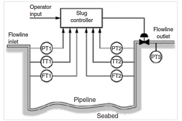
Pipeline flow measurements (FT) can be used to adjust the controller’s nominal operating point and tuning parameters.
However, large multiphase chokes often have impractical response times. The Shell Slug Suppression System (S3) overcomes this by separating fluids into gas and liquid streams in a small vessel positioned between the pipeline outlet and the main production separator. The S3 controls the liquid stream using a liquid choke and the total volumetric outflow using a smaller, more responsive gas choke, which back pressures the separator to suppress surges.
The S3 uses locally measured parameters (pressure, liquid level, flow rates) to maintain a constant total volumetric outflow, effectively suppressing severe slugging and decelerating transient slugs. This results in stabilized gas and liquid production, approximating an ideal system.
The S3 is a cost-effective alternative to traditional slug catchers, offering two key advantages: it does not cause production deferment (unlike a topside choke) and its control system is independent of downstream facilities.
Designing stable pipeline-riser systems is crucial in deepwater fields, where severe slugging is more likely and pronounced. While current slug elimination methods exist, their applicability to deepwater systems is questionable, emphasizing the need for developing new, diverse control techniques.
Real-Time Flow Assurance Monitoring
Significant efforts are underway to minimize flow assurance problems through both design and operational constraints, including procedures for shutdowns.
A real-time flow assurance monitoring system is key for optimal asset management. It continuously monitors pipeline conditions for anomalous readings (like erratic pressure fluctuations, which can indicate hydrate formation) that signal the potential formation of restrictions or blockages. Reliable, continuous, real-time data can be fed into a software simulation program for timely analysis. If an interruption occurs, this software can project where problems will arise and potentially recommend corrective actions. This rapid detection and diagnosis decreases production costs and substantially reduces the risk of environmental disasters.
The monitoring system often uses fiber optic distributed sensors to provide wide bandwidth capability and optimal data transmission rates for analysis along the pipeline. The need for these accurate and advanced distributed sensor systems is especially critical in deepwater installations, where the potential for flow assurance issues is even greater.
Multiphase Pipline Operations
After a pipeline is installed, efficient operation and automatic controls must be provided to maintain safe operation in the face of unexpected upsets. Leak detection and pigging are typically important procedures.
Leak Detection
Pipeline leaks, often caused by material or construction damage, necessitate quick detection and action to minimize spill impact. Leak detection methods fall into two categories: external and internal.
External methods include visual inspection and hydrocarbon sensing using fiber optic or dielectric cables. Internal methods, known as Computational Pipeline Monitoring (CPM), use SCADA-linked computer simulation software to continuously analyze internal parameters (flow, pressure, temperature) for unexpected variations indicating a leak.
It will be interesting: LNG Ship-to-Ship Transfer Process
The choice of method depends on pipeline and product characteristics, instrumentation, and economics. SCADA-based CPM has the widest applicability and is highly developed, rapidly detecting large leaks and eventually smaller ones.
However, applying SCADA-based CPM to multiphase flow pipelines is significantly more challenging due to the difficulty and inaccuracy of metering, mainly caused by the varying ratio of gas and liquid content and the formation of liquid slugs. Reliable flow measurement and transient flow computer models are needed for multiphase CPM. Furthermore, new technologies must be analyzed carefully for subsea pipeline application, where remoteness and complex environmental interactions make detection especially difficult.
Pigging
Pigging is a term used to describe a mechanical method for removing contaminants and deposits within the pipe or to clean accumulated liquids in the lower portions of hilly terrain pipelines using a mechanized plunger or pigs. Because of the ability of the pig to remove both corrosion products and sludge from the line, it has been found to be a positive factor in the corrosion control of Offshore terminal for transshipment of liquefied gasoffshore pipelines. Some specially instrumented pigs, known as “intelligent pigs“, may also be used intermittently for the purpose of pipeline integrity monitoring which includes detecting wall defects (e. g., corrosion, weld defects, and cracks). Pipeline pigs fit the inside diameter of the pipe and scrape the pipe walls as they are pushed along the pipeline by the flowing fluid.
For Offshore supply chain of Liquefied Natural Gasoffshore platforms the pig is launched from offshore and received in the onshore pig catcher. The receiver is in a direct line with the sealine and can be isolated from it to allow the pigs to be removed. Pigs are available in various shapes (Figure 22) and are made of different materials, depending on the pigging task to be accomplished.
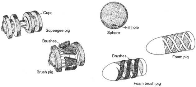
Pipeline pigs vary, including some with spring-loaded knives or brushes for contaminant removal and others that are semi-rigid, non-metallic spheres.
Pigging operations require careful control due to the lack of reliable tools for predicting pig motion. Operators must balance the risks of overfrequent pigging (high costs/downtime) and infrequent pigging (blockages/stuck pigs). Since there is no commercial tool for determining the optimum pigging frequency, operators rely on field experience and rules of thumb, which carry high uncertainty.
A significant issue in pigging is slugging, where liquid accumulates ahead of the pig, arriving as a slug at processing equipment. This causes mechanical and process problems. Operators attempt to minimize this by creating flow regimes like mist flow or by designing/equipping downstream facilities to handle slugs.
Pigging is a transient operation, with unsteady flow persisting long after the pig exits. Analyzing this transient flow behavior is crucial for designing facilities and establishing safe procedures. Simple pigging models, like Minami’s, often assume a quasi-steady gas phase, which is unsuitable for complex systems like pipeline-riser configurations due to high gas accumulation. Yeung and Lima developed a new transient two-fluid model specifically to accurately estimate two-phase flow pigging hydraulics in these complex systems.
Example 1
Using the Beggs and Brill two-phase flow correlation and the presented calculation algorithm in Figure Raw Gas Transmission: Multiphase Flow, Hydrates, and Corrosion Challenges“Pressure and temperature calculation procedure”, predict the flow temperature and pressure profiles of the Masjed Soliman to Mahshahr gas/condensate transmission line (104,4 miles long and 19-inch inside diameter) located in southwestern Iran. The pipeline elevation profile is given in Table 3.
| Table 3. Masjed Soleiman-Mahshahr Pipeline Profile | ||
|---|---|---|
| Segment number | Length (miles) | Inlet elevation (ft) |
| 1 | 7,09 | 1740,00 |
| 2 | 4,84 | 672,57 |
| 3 | 6,4 | 1197,51 |
| 4 | 3,1 | 688,98 |
| 5 | 0,62 | 1410,76 |
| 6 | 7,77 | 862,86 |
| 7 | 9,94 | 295,28 |
| 8 | 14,93 | 426,51 |
| 9 | 7,34 | 196,85 |
| 10 | 9,46 | 98,43 |
| 11 | 9,94 | 55,77 |
| 12 | 9,94 | 49,21 |
| 13 | 9,94 | 19,69 |
| 14 | 3,11 | 36,09 |
The gas composition and the pipeline data needed for all the runs are given in Tables 4 and 5, respectively.
| Table 4. Composition of Transported Gas | |
|---|---|
| Component | Mole percent |
| H2S | 25,60 |
| N2 | 0,20 |
| CO2 | 9,90 |
| C1 | 62,90 |
| C2 | 0,70 |
| C3 | 0,20 |
| iC4 | 0,06 |
| nC4 | 0,09 |
| iC5 | 0,04 |
| nC5 | 0,05 |
| C+6 | 0,26 |
Also, the parameters of the C+6 fraction are:
- molecular weight, 107,8;
- normal boiling point, 233,8 °F;
- critical temperature, 536,7 °F;
- critical pressure, 374,4 psia;
- and acentric factor, 0,3622.
| Table 5. Other Pipeline Data | |
|---|---|
| Inlet pressure, psia | 1165 |
| Inlet temperature, °F | 95 |
| Surrounding temperature, °F | 77 |
| Flow rate, MMSCFD | 180 |
| Overall heat-transfer coefficient, Btu/hr.ft2.°F | 0,25 |
Assumptions
The following assumptions will be made in the calculations required for pipeline simulation:
- this example uses the Peng and Robinson equation of state to implement the thermodynamic model, as it has proven reliable for gas/condensate systems (in conjunction with the thermodynamic model, empirical correlations for viscosity and surface tension are used);
- and the overall composition of the fluid remains constant along the pipe, which can be seen as a steady-state requirement.
Solution
The calculation algorithm presented here couples a hydrodynamic model, based on the Beggs and Brill two-phase flow correlation, to obtain the pressure profile along the pipeline and a phase behavior model, based on the Peng and Robinson equation of state, for determining the phase condition at any point in the pipe and the fluid properties. Following the procedure outlined by Brill and Beggs, the resulting algorithm allows one to predict the flow behavior of a Managing Liquefied Natural Gas Risks in the Marine Industrynatural gas/condensate system.
Figures 21 and 22 show respectively, results of the temperature and pressure profiles of the Masjed Soleiman to Mahshahr gas/condensate transmission line.
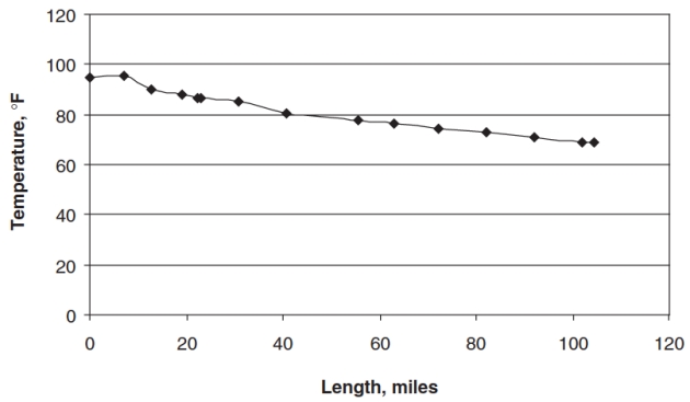
Examined case results demonstrate the ability of the Beggs and Brill introduced algorithm (Figure Raw Gas Transmission: Multiphase Flow, Hydrates, and Corrosion Challenges“Pressure and temperature calculation procedure”) to predict the pressure and temperature gradients at any point in the pipe.
Note
The Masjed Soleiman to Mahshahr pipeline was intended to operate as a single-phase gas line and was designed on that basis. However, operation of the line clearly showed liquid to be present. This occurs when the pressure and the temperature changes traverse the two-phase region of the phase envelope such that the system changes from single phase to two phase. As the system enters the two-phase region, mass transfer between gas and liquid phases causes condensation and gives rise to two-phase flow in the pipeline. This example shows how the Pipelines in Marine Terminals: Key Considerations for Handling Liquefied Gasgas pipeline designer has to use phase behavior analysis as an operational tool in order to predict the presence of liquid in the system. Phase behavior analysis is conducted to determine the bubble and dew point curve and to perform flash calculations at any pressure and temperature. Then the operational pressure-temperature profile is overplotted on the phase envelope diagram in order to evaluate the condensation possibility into the gas pipeline.
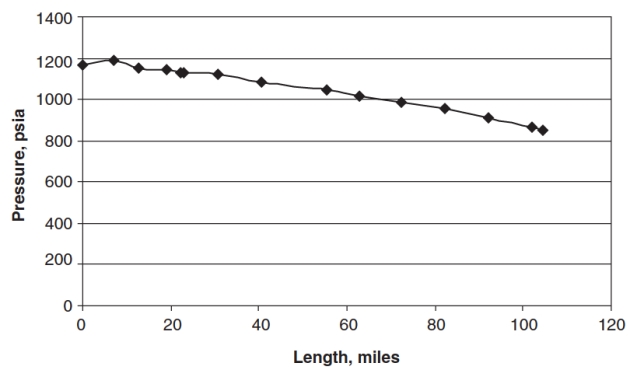
When thermodynamic conditions dictate single-phase gas flow, the single-phase flow equations should be applied instead of two-phase flow models. However, in this case, the Beggs and Brill two-phase flow correlation (neglecting the liquid holdup parameter in all of calculations) was used to estimate pressure drop for pipe segments containing no liquid.
Example 2
Estimate the hydrate formation temperature for the following mixture at 661,37 psia using the Katz gravity chart, Towler and Mokhatab correlation, and Baillie and Wichert chart (the experimentally observed value is 57,56 °F).
- CH4 82,0 mol%.
- CO2 12,6 mol%.
- H2S 5,4 mol%.
Solution
Calculate the molar mass and gravity of the gas mixture:
Therefore, SG = 20,541/28,966 = 0,709.
- Using the Katz gravity chart: Th = 59 °F.
- Using the Towler and Mokhatab correlation [Equation 4] representing the Katz gravity chart:
To use the Baillie and Wichert method to estimate the hydrate formation temperature, enter the main chart at the given pressure and then move to the right to the appropriate H2S concentration. From that point, go straight down to the appropriate gas-specific gravity. Then follow the sloping lines down to the temperature axis. This value is the based temperature. In this case, the base temperature is about 66 °F. Now go to the temperature correction in the upper left. Enter the chart with the H2S concentration and move across to the appropriate propane concentration. From that point, go straight down to the appropriate pressure curve and then read the temperature correction from the left or the right axis, depending on the position in the pressure section. In this case, the temperature correction is negative (-7 °F) because it comes from the left half of the correction chart. Finally, the hydrate formation temperature is obtained by adding the temperature correction to the base temperature, 59 °F.
Example 3
Natural gas flowing at 4 MMscfd is transferred through a pipeline from a well site to a Liquefied Natural Gas Plant and Regasification Terminal Operationsprocessing plant. The production also includes 7,062 scfd of water, which is transferred in the same pipeline. The inlet pressure and temperature are 1 165 psia and 95 °F, respectively. The hydrate formation temperature of the gas is determined to be 84,485 °F at stream pressure.
In transportation through the pipeline, the gas is expected to cool to 48,92 °F. Calculate the amount of methanol that should be injected into the line in order to prevent hydrate formation.
Solution
1 Calculate the required temperature depression:
2 Use Equation 5 to estimate the concentration of methanol required to yield the desired temperature depression:
Because this is outside the range of applicability of the Hammerschmidt equation, this result should be taken with some caution. However, the value obtained from the Nielsen and Bucklin equation [Equation 6] is Xmethanol = 0,2399, and then to calculate the weight percent from this mole fraction, the following equation is used:
3 Calculate the amount of methanol required to get a 35,952 wt % solution based on water and methanol:
Therefore, methanol mass flow rate = 247,439 lbm/day. The density of methanol is 49,717 lbm/ft3, so the methanol is injected at a rate of 4,976 ft3/day.
Read also: Understanding LNG Tank Atmosphere and Material Properties: Key Principles for Safety and Efficiency
Note that the amount of water in the natural gas has been neglected in this calculation, where the gas is being produced with free water, so it can be assumed that is saturated with water. However, to estimate the amount of methanol required to saturate the gas, Figure 8 can be used.
From that figure and then estimating the amount of methanol in the vapor phase, the total methanol requirement will be determined.

- Acikgoz, M., Franca, F., and Lahey Jr, R. T., An experimental study of three-phase flow regimes. Int. J. Multiphase Flow 18(3), 327-336 (1992).
- Adewmi, M. A., and Bukacek, R. F., Two-phase pressure drop in horizontal pipelines. J. Pipelines 5, 1-14 (1985).
- Amdal, J., et al., “Handbook of Multiphase Metering.” Produced for The Norwegian Society for Oil and Gas Measurement, Norway (2001).
- Ansari, A. M., Sylvester, A. D., Sarica, C., Shoham, O., and Brill, J. P., A comprehensive mechanistic model for upward two-phase flow in wellbores. SPE Prod. Facilit. J. 143-152 (May 1994).
- API, “Computational Pipeline Monitoring”. API Publication 1130, 17, American Petroleum Institute, TX (1995a).
- API, “Evaluation Methodology for Software Based Leak Detection Systems”. API Publication 1155, 93, American Petroleum Institute, TX (1995b).
- API RP 14E, “Recommended Practice for Design and Installation of Offshore Production Platform Piping Systems”, 5th Ed., p. 23.
- Asante, B., “Two-Phase Flow: Accounting for the Presence of Liquids in Gas Pipeline Simulation”. Paper presented at 34th PSIG Annual Meeting, Portland, Oregon (Oct. 23–25, 2002).
- AsphWax’s Flow Assurance course, “Fluid Characterization for Flow Assurance”. AsphWax Inc., Stafford, TX (2003).
- Ayala, F. L., and Adewumi, M. A., Low-liquid loading multiphase flow in natural gas pipelines. ASME J. of Energy Res. Technol. 125, 284-293 (2003).
- Baillie, C., and Wichert, E., Chart gives hydrate formation temperature for natural gas. Oil Gas J. 85(4), 37-39 (1987).
- Baker, O., Design of pipelines for simultaneous flow of oil and gas. Oil Gas J. 53, 185 (1954).
- Banerjee, S., “Basic Equations”. Lecture presented at the Short Course on Modeling of Two-Phase Flow Systems, ETH Zurich, Switzerland (March 17-21, 1986).
- Barnea, D., A unified model for prediction flow pattern transitions for the whole range of pipe inclinations. Int. J. Multiphase Flow 13(1), 1-12 (1987).
- Barnea, D., and Taitel, Y., Stratified three-phase flow in pipes: Stability and transition. Chem. Eng. Comm. 141–142, 443-460 (1996).
- Battara, V., Gentilini, M., and Giacchetta, G., Condensate-line correlations for calculating holdup, friction compared to field data. Oil Gas J. 30, 148–52 (1985).
- Bay, Y., “Pipelines and Risers”, Vol. 5. Elsevier Ocean Engineering Book Series (2001).
- Beggs, H. D., and Brill, J. P., “A Study of Two-Phase Flow in Inclined Pipes”. JPT, 607-17; Trans., AIME, 255 (May 1973).
- Bendiksen, K., Brandt, I., Jacobsen, K. A., and Pauchon, C., “Dynamic Simulation of Multiphase Transportation Systems”. Multiphase Technology and Consequence for Field Development Forum, Stavanger, Norway (1987).
- Bendiksen, K., Malnes, D., Moe, R., and Nuland, S., The dynamic two-fluid model OLGA: Theory and application. SPE Prod. Eng. 6, 171-180 (1991).
- Bertola, V., and Cafaro, E., “Statistical Characterization of Subregimes in Horizontal Intermittent Gas/Liquid Flow”. Proc. the 4th International Conference on Multiphase Flow, New Orleans, LA (2001).
- Bjune, B., Moe, H., and Dalsmo, M., Upstream control and optimization increases return on investment. World Oil 223, 9 (2002).
- Black, P. S., Daniels, L. C., Hoyle, N. C., and Jepson, W. P., Studying transient multiphase flow using the pipeline analysis code (PLAC). ASME J. Energy Res. Technol. 112, 25-29 (1990).
- Bloys, B., Lacey, C., and Lynch, P., “Laboratory Testing and Field Trial of a New Kinetic Hydrate Inhibitor”. Proc. 27th Annual Offshore Technology Conference, OTC 7772, PP. 691-700, Houston, TX (1995).
- Bonizzi, M., and Issa, R. I., On the simulation of three-phase slug flow in nearly horizontal pipes using the multi-fluid model. Int. J. Multiphase Flow 29, 1719-1747 (2003).
- Boriyantoro, N. H., and Adewumi, M. A., “An Integrated Single-Phase/Two-Phase Flow Hydrodynamic Model for Predicting the Fluid Flow Behavior of Gas Condensate Pipelines”. Paper presented at 26th PSIG Annual Meeting, San Diego, CA (1994).
- Brauner, N., and Maron, M. D., Flow pattern transitions in two-phase liquid-liquid flow in horizontal tubes, Int. J. Multiphase Flow 18, 123-140 (1992).
- Brauner, N., The prediction of dispersed flows boundaries in liquid-liquid and gas-liquid systems, Int. J. Multiphase Flow 27, 885-910 (2001).
- Brill, J. P., and Beggs, H. D., “Two-Phase Flow in Pipes”, 6th Ed. Tulsa University Press, Tulsa, OK (1991).
- Bufton, S. A., Ultra Deepwater will require less conservative flow assurance approaches. Oil Gas J. 101(18), 66-77 (2003).
- Campbell, J. M., “Gas Conditioning and Processing”, 3rd Ed. Campbell Petroleum Series, Norman, OK (1992).
- Carroll, J. J., “Natural Gas Hydrates: A Guide for Engineers”. Gulf Professional Publishing, Amsterdam, The Netherlands (2003).
- Carroll, J. J., “An Examination of the Prediction of Hydrate Formation Conditions in Sour Natural Gas”. Paper presented at the GPA Europe Spring Meeting, Dublin, Ireland (May 19-21, 2004).
- Carson, D. B., and Katz, D. L., Natural gas hydrates. Petroleum Trans. AIME 146, 150-158 (1942).
- Chen, C. J., Woo, H. J., and Robinson, D. B., “The Solubility of Methanol or Glycol in Water-Hydrocarbon Systems”. GPA Research Report RR-117, Gas Processors Association, OK (March 1988).
- Chen, X., and Guo, L., Flow patterns and pressure drop in oil-air-water three-phase flow through helically coiled tubes. Int. J. Multiphase Flow 25, 1053-1072 (1999).
- Cheremisinoff, N. P., “Encyclopedia of Fluid Mechanics”, Vol. 3. Gulf Professional Publishing, Houston, TX (1986).
- Chisholm, D., and Sutherland, L. A., “Prediction of Pressure Gradient in Pipeline Systems during Two-Phase Flow”. Paper presented at Symposium on Fluid Mechanics and Measurements in Two-Phase Flow Systems, Leeds (Sept. 1969).
- Cindric, D. T., Gandhi, S. L., and Williams, R. A., “Designing Piping Systems for Two-Phase Flow”. Chem. Eng. Progress, 51-59 (March 1987).
- Collier, J. G., and Thome, J. R., “Convective Boiling and Condensation”, 3rd Ed. Clarendon Press, Oxford, UK (1996).
- Colson, R., and Moriber, N. J., Corrosion control. Civil Eng. 67(3), 58-59 (1997).
- Copp, D. L., “Gas Transmission and Distribution”. Walter King Ltd., London (1970).
- Courbot, A., “Prevention of Severe Slugging in the Dunbar 16 Multiphase Pipelines”. Paper presented at the Offshore Technology Conference, Houston, TX (May 1996).
- Covington, K. C., Collie, J. T., and Behrens, S. D., “Selection of Hydrate Suppression Methods for Gas Streams”. Paper presented at the 78th GPA Annual Convention, Nashville, TN (1999).
- Cranswick, D., “Brief Overview of Gulf of Mexico OCS Oil and Gas Pipelines: Installation, Potential Impacts, and Mitigation Measures”. U. S. Department of the Interior, Minerals Management Service, Gulf of Mexico OCS Region, New Orleans, LA (2001).
- Dhl, E., et al., “Handbook of Water Fraction Metering”, Rev. 1. Norwegian Society for Oil and Gas Measurements, Norway (June 2001).
- Decarre, S., and Fabre, J., Etude Sur La Prediction De l’Inversion De Phase. Revue De l’Institut Francais Du Petrole 52, 415-424 (1997).
- De Henau, V., and Raithby, G. D., A transient two-fluid model for the simulation of slug flow in pipelines. Int. J. Multiphase Flow 21, 335–349 (1995).
- Dukler, A. E., “Gas-Liquid Flow in Pipelines Research Results”. American Gas Assn. Project NX-28 (1969).
- Dukler, A. E., and Hubbard, M. G., “The Characterization of Flow Regimes for Horizontal Two-Phase Flow”. Proc. Heat Transfer and Fluid Mechanics Institute, 1, 100-121, Stanford University Press, Stanford, CA (1966).
- Eaton, B. A., et al., The prediction of flow pattern, liquid holdup and pressure losses occurring during continuous two-phase flow in horizontal pipelines. J. Petro. Technol. 240, 815-28 (1967).
- Edmonds, B., et al., “A Practical Model for the Effect of Salinity on Gas Hydrate Formation”. European Production Operations Conference and Exhibition, Norway (April 1996).
- Edmonds, B., Moorwood, R. A. S., and Szczepanski, R., “Hydrate Update”. GPA Spring Meeting, Darlington (May 1998).
- Esteban, A., Hernandez, V., and Lunsford, K., “Exploit the Benefits of Methanol”. Paper presented at the 79th GPA Annual Convention, Atlanta, GA (2000).
- Fabre, J., et al., Severe slugging in pipeline/riser systems. SPE Prod. Eng. 5(3), 299-305 (1990).
- Faille, I., and Heintze, E., “Rough Finite Volume Schemes for Modeling Two-Phase Flow in a Pipeline”. In Proceeding of the CEA.EDF.INRIA Course, INRIA Rocquencourt, France (1996).
- Fidel-Dufour, A., and Herri, J. S., “Formation and Dissociation of Hydrate Plugs in a Water in Oil Emulsion”. Paper presented at the 4th International Conference on Gas Hydrates, Yokohama, Japan (2002).
- Frostman, L. M., “Anti-aggolomerant Hydrate Inhibitors for Prevention of Hydrate Plugs in Deepwater Systems”. Paper presented at the SPE Annual Technical Conference and Exhibition, Dallas, TX (Oct. 1-4, 2000).
- Frostman, L. M., et al., “Low Dosage Hydrate Inhibitors (LDHIs): Reducing Total Cost of Operations in Existing Systems and Designing for the Future”. Paper presented at the SPE International Symposium on Oilfield Chemicals, Houston, TX (Feb. 5-7, 2003).
- Frostman, L. M., “Low Dosage Hydrate Inhibitor (LDHI) Experience in Deepwater”. Paper presented at the Deep Offshore Technology Conference, Marseille, France (Nov. 19-21, 2003).
- Fuchs, P., “The Pressure Limit for Terrain Slugging”. Proceeding of the 3rd BHRA International Conference on Multiphase Flow, Hague, The Netherlands (May 1987).
- Furlow, W., “Suppression System Stabilizes Long Pipeline-Riser Liquid Flows”. Offshore, Deepwater D&P, 48 + 166 (Oct., 2000).
- Giot, M., “Three-Phase Flow”, Chap. 7.2. McGraw-Hill, New York (1982).
- Goulter, D., and Bardon, M., Revised equation improves flowing gas temperature prediction. Oil Gas J. 26, 107-108 (1979).
- Govier, G. W., and Aziz, K., “The Flow of Complex Mixtures in Pipes”. Van Nostrand Reinhold Co., Krieger, New York (1972).
- GPSA Engineering Data Book, 11th Ed. Gas Processors Suppliers Association, Tulsa, OK (1998).
- Gregory, G. A., and Aziz, K., Design of pipelines for multiphase gas-condensate flow. J. Can. Petr. Technol. 28-33 (1975).
- Griffith, P., and Wallis, G. B., Two-phase slug flow. J. Heat Transfer Trans. ASME. 82, 307-320 (1961).
- Haandrikman, G., Seelen, R., Henkes, R., and Vreenegoor, R., “Slug Control in Flowline/Riser Systems”. Paper presented at the 2nd International Conference on Latest Advance in Offshore Processing, Aberdeen, UK (Nov. 9-10, 1999).
- Hall, A. R. W., “Flow Patterns in Three-Phase Flows of Oil, Water, and Gas”. Paper presented at the 8th BHRG International Conference on Multiphase Production, Cannes, France (1997).
- Hammerschmidt, E. G., Formation of gas hydrates in natural gas transmission lines. Ind. Eng. Chem. 26, 851-855 (1934).
- Hart, J., and Hamersma P. J. Correlations predicting frictional pressure drop and liquid holdup during horizontal gas-liquid pipe flow with small liquid holdup. Int. J. Multiphase Flow 15(6), 974-964 (1989).
- Hartt, W. H., and Chu, W., New methods for CP design offered. Oil Gas J. 102(36), 64-70 (2004).
- Hasan, A. R., Void fraction in bubbly and slug flow in downward two-phase flow in vertical and inclined wellbores, SPE Prod. Facil. 10(3), 172–176 (1995).
- Hasan, A. R., and Kabir, C. S., “Predicting Multiphase Flow Behavior in a Deviated Well”. Paper presented at the 61st SPE Annual Technical Conference and Exhibition, New Orleans, LA (1986).
- Hasan, A. R., and Kabir, C. S., Gas void fraction in two-phase up-flow in vertical and inclined annuli. Int. J. Multiphase Flow 18(2), 279-293 (1992).
- Hasan, A. R., and Kabir, C. S., Simplified model for oil/water flow in vertical and deviated wellbores. SPE Prod. Facil. 14(1), 56-62 (1999).
- Hasan, A. R., and Kabir, C. S., “Fluid and Heat Transfers in Wellbores”. Society of Petroleum Engineers (SPE) Publications, Richardson, TX (2002).
- Havre, K., and Dalsmo, M., “Active Feedback Control as the Solution to Severe Slugging”. Paper presented at the SPE Annual Technical Conference and Exhibition, New Orleans, LA (Oct. 3, 2001).
- Havre, K., Stornes, K., and Stray, H., “Taming Slug Flow in Pipelines”. ABB Review No. 4, 55-63, ABB Corporate Research AS, Norway (2000).
- Hedne, P., and Linga, H., “Suppression of Terrain Slugging with Automatic and Manual Riser Chocking”. Advances in Gas-Liquid Flows, 453-469 (1990).
- Hein, M., “HP41 Pipeline Hydraulics and Heat Transfer Programs.” PennWell Publishing Company, Tulsa, OK (1984).
- Henriot, V., Courbot, A., Heintze, E., and Moyeux, L., “Simulation of Process to Control Severe Slugging: Application to the Dunbar Pipeline”. Paper presented at the SPE Annual Conference and Exhibition, Houston, TX (1999).
- Hewitt, G. F., and Roberts, D. N., “Studies of Two-Phase Flow Patterns by Simultaneous X-ray and Flash Photography”. AERE-M 2159, HMSO (1969).
- Hill, T. H., Gas injection at riser base solves slugging, flow problems. Oil Gas J. 88(9), 88-92 (1990).
- Hill, T. J., “Gas-Liquid Challenges in Oil and Gas Production”. Proceeding of ASME Fluids Engineering Division Summer Meeting, Vancouver, BC, Canada (June 22-26, 1997).
- Holt, A. J., Azzopardi, B. J., and Biddulph, M. W., “The Effect of Density Ratio on Two-Phase Frictional Pressure Drop”. Paper presented at the 1st International Symposium on Two-Phase Flow Modeling and Experimentation, Rome, Italy (Oct. 9-11, 1995).
- Holt, A. J., Azzopardi, B. J., and Biddulph, M. W., Calculation of two-phase pressure drop for vertical up flow in narrow passages by means of a flow pattern specific models. Trans. IChemE 77(Part A), 7-15 (1999).
- Hunt, A., Fluid properties determine flow line blockage potential. Oil Gas J. 94(29), 62–66 (1996).
- IFE, “Mitigating Internal Corrosion in Carbon Steel Pipelines”. Institute of Energy Technology News, Norway (April 2000).
- Jansen, F. E., Shoham, O., and Taitel, Y., The elimination of severe slug-ging, experiments and modeling. Int. J. Multiphase Flow 22(6), 1055-1072 (1996).
- Johal, K. S., et al., “An Alternative Economic Method to Riser Base Gas Lift for Deepwater Subsea Oil/Gas Field Developments”. Proceeding of the Offshore Europe Conference, 487-492, Aberdeen, Scotland (9-12 Sept., 1997).
- Jolly, W. D., Morrow, T. B., O’Brien, J. F., Spence, H. F., and Svedeman, S. J., “New Methods for Rapid Leak Detection in Offshore Pipelines”. Final Report, SWRI Project No. 04-4558, SWRI (April 1992).
- Jones, O. C., and Zuber, N., The interrelation between void fraction fluctuations and flow patterns in two-phase flow Int. J. Multiphase Flow. 2, 273-306 (1975).
- Kang, C., Wilkens, R. J., and Jepson, W. P., “The Effect of Slug Frequency on Corrosion in High-Pressure, Inclined Pipelines”. Paper presented at the NACE International Annual Conference and Exhibition, Paper No. 96020, Denver, CO (March 1996).
- Katz, D. L., Prediction of conditions for hydrate formation in natural gases. Trans. AIME 160, 140–149 (1945).
- Kelland, M. A., Svartaas, T. M., and Dybvik, L., “New Generation of Gas Hydrate Inhibitors”. 70th SPE Annual Technical Conference and Exhibition, 529-537, Dallas, TX (Oct. 22-25, 1995).
- Kelland, M. A., Svartaas, T. M., Ovsthus, J., and Namba, T., A new class of kinetic inhibitors. Ann. N. Y. Acad. Sci. 912, 281-293 (2000).
- King, M. J. S, “Experimental and Modelling Studies of Transient Slug Flow”. Ph.D. Thesis, Imperial College of Science, Technology, and Medicine, London, UK (March 1998).
- Klemp, S., “Extending the Domain of Application of Multiphase Technology”. Paper presented at the 9th BHRG International Conference on Multiphase Technology, Cannes, France (June 16-18, 1999).
- Kohl, A. L., and Risenfeld, F. C., “Gas Purification.” Gulf Professional Publishing, Houston, TX (1985).
- Kovalev, K., Cruickshank, A., and Purvis, J., “Slug Suppression System in Operation”. Paper presented at the 2003 Offshore Europe Conference, Aberdeen, UK (Sept. 2-5, 2003).
- Kumar, S., “Gas Production Engineering”. Gulf Professional Publishing, Houston, TX (1987).
- Lagiere, M., Miniscloux, and Roux, A., Computer two-phase flow model predicts pipeline pressure and temperature profiles. Oil Gas J. 82-91 (April 9, 1984).
- Langner, et al., “Direct Impedance Heating of Deepwater Flowlines.” Paper presented at the Offshore Technology Conference (OTC), Houston, TX (1999).
- Lederhos, J. P., Longs, J. P., Sum, A., Christiansen, R. l., and Sloan, E. D., Effective kinetic inhibitors for natural gas hydrates. Chem. Eng. Sci. 51(8), 1221-1229 (1996).
- Lee, H. A., Sun, J. Y., and Jepson, W. P., “Study of Flow Regime Transitions of Oil-Water-Gas Mixture in Horizontal Pipelines”. Paper presented at the 3rd International Offshore and Polar Engng Conference, Singapore (June 6–11 1993).
- Leontaritis, K. J., “The Asphaltene and Wax Deposition Envelopes”. The Symposium on Thermodynamics of Heavy Oils and Asphaltenes, Area 16C of Fuels and Petrochemical Division, AIChE Spring National Meeting and Petroleum Exposition, Houston, TX (March 19-23, 1995).
- Leontaritis, K. J., “PARA-Based (Paraffin-Aromatic-Resin-Asphaltene) Reservoir Oil Characterization”. Paper presented at the SPE International Symposium on Oilfield Chemistry, Houston, TX (Feb. 18-21, 1997a).
- Leontaritis, K. J., Asphaltene destabilization by drilling/completion fluids. World Oil 218(11), 101-104 (1997b).
- Leontaritis, K. J., “Wax Deposition Envelope of Gas Condensates”. Paper presented at the Offshore Technology Conference (OTC), Houston, TX (May 4–7 1998).
- Lin, P. Y., and Hanratty, T. J., Detection of slug flow from pressure measurements. Int. J. Multiphase Flow 13, 13-21 (1987).
- Lockhart, R. W., and Martinelli, R. C., Proposed correlation of data for isothermal two-phase, two-component flow in pipes. Chem. Eng. Prog. 45, 39-48 (1949).
- Maddox, R. N., et al., “Predicting Hydrate Temperature at High Inhibitor Concentration”. Proceedings of the Laurance Reid Gas Conditioning Conference, 273-294, Norman, OK (1991).
- Mann, S. L., et al., “Vapour-Solid Equilibrium Ratios for Structure I and II Natural Gas Hydrates”. Proceedings of the 68th GPA Annual Convention, 60-74, San Antonio, TX (March 13-14, 1989).
- Martinelli, R. C., and Nelson, D. B., Prediction of pressure drop during forced circulation boiling of water. Trans. ASME 70, 695 (1948).
- Masella, J. M., Tran, Q. H., Ferre, D., and Pauchon, C., Transient simulation of two-phase flows in pipes. Oil Gas Sci. Technol. 53(6), 801–811 (1998).
- McCain, W. D., “The Properties of Petroleum Fluids”, 2nd Ed. Pennwell Publishing Company, Tulsa, OK (1990).
- McLaury, B. S., and Shirazi, S. A., An alternative method to API RP 14E for predicting solids erosion in multiphase flow. ASME J. Energy Res. Technol. 122, 115-122 (2000).
- McLeod, H. O., and Campbell, J. M., Natural gas hydrates at pressure to 10,000 psia. J. Petro. Technol. 13, 590-594 (1961).
- Mehta, A. P., and Sloan, E. D., “Structure H Hydrates: The State-of-the-Art”. Paper presented at the 75th GPA Annual Convention, Denver, CO (1996).
- Mehta, A., Hudson, J., and Peters, D., “Risk of Pipeline Over-Pressurization during Hydrate Remediation by Electrical Heating”. Paper presented at the Chevron Deepwater Pipeline and Riser Conference, Houston, TX (March 28-29, 2001).
- Mehta, A. P., Hebert, P. B., and Weatherman, J. P., “Fulfilling the Promise of Low Dosage Hydrate Inhibitors: Journey from Academic Curiosity to Successful Field Implementations”. Paper presented at the 2002 Offshore Technology Conference, Houston, TX (May 6-9, 2002).
- Minami, K., “Transient Flow and Pigging Dynamics in Two-Phase Pipelines”. Ph.D. Thesis, University of Tulsa, Tulsa, OK (1991).
- Mokhatab, S., Correlation predicts pressure drop in gas-condensate pipelines. Oil Gas J. 100(4), 66-68 (2002a).
- Mokhatab, S., New correlation predicts liquid holdup in gas-condensate pipelines. Oil Gas J. 100(27), 68-69 (2002b).
- Mokhatab, S., Model aids design of three-phase, gas-condensate transmission lines. Oil Gas J. 100(10), 60-64 (2002c).
- Mokhatab, S., Three-phase flash calculation for hydrocarbon systems containing water. J. Theor. Found. Chem. Eng. 37(3), 291-294 (2003).
- Mokhatab, S., Upgrade velocity criteria for sizing multiphase pipelines. J. Pipeline Integrity 3(1), 55-56 (2004).
- Mokhatab, S., “Interaction between Multiphase Pipelines and Down-stream Processing Plants”. Report No. 3, TMF3 Sub-Project VII: Flexible Risers, Transient Multiphase Flow (TMF) Program, Cranfield University, Bedfordshire, England (May 2005).
- Mokhatab, S., “Explicit method predicts temperature and pressure profiles of gas-condensate pipelines”. Accepted for publication in Energy Sources: Part A (2006a).
- Mokhatab, S., Severe slugging in a catenary-shaped riser: Experimental and simulation studies”. Accepted for publication in J. Petr. Sci. Technol. (2006b).
- Mokhatab, S., Dynamic simulation of offshore production plants. Accepted for publication in J. Petr. Sci. Technol. (2006c).
- Mokhatab, S., Severe slugging in flexible risers: Review of experimental investigations and OLGA predictions. Accepted for publication in J. Petro. Sci. Technol. (2006d).
- Mokhatab, S., and Bonizzi, M., “Model predicts two-phase flow pressure drop in gas-condensate transmission lines”. Accepted for publication in Energy Sources: Part A (2006).
- Mokhatab, S., Towler, B. F., and Purewal, S., A review of current technologies for severe slugging remediation”. Accepted for publication in J. Petro. Sci. Technol. (2006a).
- Mokhatab, S., Wilkens, R. J., and Leontaritis, K. J., “A Review of strategies for solving gas hydrate problems in subsea pipelines”. Accepted for publication in Energy Sources: Part A (2006b).
- Molyneux, P., Tait, A., and Kinving, J., “Characterization and Active Control of Slugging in a Vertical Riser”. Proceeding of the 2nd North American Conference on Multiphase Technology, 161–170, Banff, Canada (June 21–23, 2000).
- Moody, L. F., Friction factors for pipe flow. Trans. ASME 66, 671–684 (1944).
- Mucharam, L., Adewmi, M. A., and Watson, R., Study of gas condensation in transmission pipelines with a hydrodynamic model. SPE J. 236–242 (1990).
- Muhlbauer, K. W., “Pipeline Risk Management Manual”, 2nd Ed. Gulf Professional Publishing, Houston, TX (1996).
- Narayanan, L., Leontaritis, K. J., and Darby, R., “A Thermodynamic Model for Predicting Wax Precipitation from Crude Oils”. The Symposium of Solids Deposition, Area 16C of Fuels and Petro-chemical Division, AIChE Spring National Meeting and Petroleum Exposition, Houston, TX (March 28-April 1, 1993).
- Nasrifar, K., Moshfeghian, M., and Maddox, R. N., Prediction of equilibrium conditions for gas hydrate formation in the mixture of both electrolytes and alcohol. Fluid Phase Equilibria 146, 1–2, 1–13 (1998).
- National Association of Corrosion Engineers, “Sulfide Stress Cracking Resistant Metallic Materials for Oil Field Equipment”. NACE Std MR-01-75 (1975).
- Ng, H. J., and Robinson, D. B., The measurement and prediction of hydrate formation in liquid hydrocarbon-water systems. Ind. Eng. Chem. Fund. 15, 293-298 (1976).
- Nielsen, R. B., and Bucklin, R. W., Why not use methanol for hydrate control? Hydrocarb. Proc. 62(4), 71-78 (1983).
- Nyborg, R., Corrosion control in oil and gas pipelines. Business Briefing Exploration Prod. Oil Gas Rev. 2, 79-82 (2003).
- Oram, R. K., “Advances in Deepwater Pipeline Insulation Techniques and Materials”. Deepwater Pipeline Technology Congress, London, UK (Dec. 11–12, 1995).
- Oranje, L., Condensate behavior in gas pipelines is predictable. Oil Gas J. 39 (1973).
- Osman, M. E., and El-Feky, S. A., Design methods for two-phase pipelines compared, evaluated. Oil Gas J. 83(35), 57-62 (1985).
- Palermo, T., Argo, C. B., Goodwin, S. P., and Henderson, A., Flow loop tests on a novel hydrate inhibitor to be deployed in North Sea ETAP field. Ann. N. Y. Acad. Sci. 912, 355–365, (2000).
- Pan, L., “High Pressure Three-Phase (Gas/Liquid/Liquid) Flow”. Ph. D. Thesis, Imperial College, London (1996).
- Patault, S., and Tran, Q. H., “Modele et Schema Numerique du Code TACITE-NPW”. Technical Report 42415, Institut Francais du Petrole, France (1996).
- Pauchon, C., Dhulesia, H., Lopez, D., and Fabre, J., “TACITE: A Comprehensive Mechanistic Model for Two-Phase Flow”. Paper presented at the 6th BHRG International Conference on Multiphase Production, Cannes, France (1993).
- Pauchon, C., Dhulesia, H., Lopez, D., and Fabre, J., “TACITE: A Transient Tool for Multiphase Pipeline and Well Simulation”. Paper presented at the SPE Annual Technical Conference and Exhibition, New Orleans, LA (1994).
- Peng, D., and Robinson, D. B., A new two-constant equation of state. Ind. Eng. Chem. Fundam. 15(1), 59-64 (1976).
- Petalas, N., and Aziz, K., A mechanistic model for multiphase flow in pipes. J. Can. Petr. Technol. 39, 43-55 (2000).
- Polignano, R., Value of glass-fiber fabrics proven for bituminous coatings. Oil Gas J. 80(41), 156–158, 160 (1982).
- Pots, B. F. M., et al., “Severe Slug Flow in Offshore Flowline/Riser Systems”. Paper presented at the SPE Middle East Oil Technical Conference and Exhibition, Bahrain (March 11–14, 1985).
- Rajkovic, M., Riznic, J. R., and Kojasoy, G., “Dynamic Characteristics of Flow Pattern Transitions in Horizontal Two-Phase Flow”. Proc. 2nd European Thermal Science and 14th UIT National Heat Transfer Conference, 3, 1403–1408, Edizioni ETS, Pisa, Italy (1996).
- Ramachandran, S., Breen, P., and Ray, R., Chemical programs assure flow and prevent corrosion in deepwater facilities and dlowlines. InDepth 6, 1 (2000).
- Rhodes, K. I., Pipeline protective coatings used in saudi Arabia. Oil Gas J. 80(31), 123–127 (1982).
- Ripmeester, J. A., Tse, J. S., Ratcliffe, C. J., and McLaurin, G. E., Nature 135, 325 (1987).
- Sagatun, S. I., Riser slugging: A mathematical model and the practical consequences. SPE Product. Facil. J. 19(3), 168–175 (2004).
- Salama, M. M., An alternative to API 14E erosional velocity limits for sand-laden fluids. ASME J. Energy Res. Technol. 122, 71–77 (2000).
- Samant, A. K., “Corrosion Problems in Oil Industry Need More Attention”. Paper presented at ONGC Library, Oil and Natural Gas Corporation Ltd. (Feb. 2003).
- Sandberg, C., Holmes, J., McCoy, K., and Koppitsch, H., The application of a continues leak detection system to pipelines and associated equipment. IEEE Transact. Indust. Appl. 25, 5 (1989).
- Sarica, C., and Shoham, O., A simplified transient model for pipeline/riser systems. Chem. Engi. Sci. 46(9), 2167–2179 (1991).
- Sarica, C., and Tengesdal, J. Q., A New Technique to Eliminate Severe Slugging in Pipeline/Riser Systems”. Paper presented at the 75th SPE Annual Technical Conference and Exhibition, Dallas, TX (Oct. 1–4, 2000).
- Schmidt, Z., “Experimental Study of Two-Phase Slug Flow in a Pipeline-Riser System.” Ph.D. Dissertation, University of Tulsa, Tulsa, OK (1977).
- Schmidt, Z., Brill, J. P., and Beggs, D. H., Experimental study of severe slugging in a two-phase flow pipeline-riser system. SPE J. 20, 407–414 (1980).
- Schmidt, Z., Doty, D. R., and Dutta-Roy, K., Severe slugging in offshore pipeline-riser systems. SPE J. 27–38 (1985).
- Schweikert, L. E., Tests prove two-phase efficiency for offshore pipeline. Oil Gas J. 39-42 (1986).
- Scott, S. L., Brill, J. P., Kuba, G. E., Shoham, K. A., and Tam, W., “Two-Phase Flow Experiments in the Prudhoe Bay Field of Alaska”. Paper presented at the Multiphase Flow Technology and Consequences for Field Development Conference, 229–251, Stavanger, Norway (1987).
- Shoham, O., “Flow Pattern Transitions and Characterization in Gas-Liquid Two Phase Flow in Inclined Pipes”. Ph. D. Thesis, Tel-Aviv University, Ramat-Aviv, Israel (1982).
- Sinquin, A., Palermo, T., and Peysson, Y., Rheological and flow properties of gas hydrate suspensions. Oil Gas Sci. Technolo. Rev. IFP. 59(1), 41–57 (2004).
- Sloan, E. D., Jr., Natural gas hydrates. J. Petro. Technol. 43, 1414 (1991).
- Sloan, E. D., Jr., “Clathrate Hydrates of Natural Gases”, 2nd Ed. Dekker, New York (1998).
- Sloan, E. D., Jr., “Hydrate Engineering”. SPE Monograph, 21, Society of Petroleum Engineers (SPE) Publications, Richardson, TX (2000).
- Smart, J., A method for calculating the corrosion allowance for deepwater pipelines and risers. J. Pipeline Integrity 73 (2001).
- Soldati, A., Paglianti, A., and Giona, M., Identification of two-phase flow regimes via diffusional analysis of experimental time series. Exp. Fluids 21, 151–160 (1996).
- Son, V. K., and Wallace, C., “Reclamation/Regeneration of Glycols Used for Hydrate Inhibition”. Paper presented at the 12th Annual Deep Offshore Technology Conference and Exhibition, New Orleans, LA (Nov. 7–9, 2000).
- Sotberg, T., and Bruschi, R., “Future Pipeline Design Philosophy-Framework”. Paper presented at the 11th International Conference on Offshore Mechanics and Arctic Engineering, Calgary, AB, Canada (1992).
- Storkaas, E., Alstad, V., and Skogestad, S., “Stabilization of Desired Flow Regimes in Pipelines”. Paper presented at the AIChE Annual Meeting, Reno, NV (2001).
- Strommen, R. D., Horn, H., and Wold, K. R., New technique monitors pipeline corrosion, cracking. Oil Gas J. 91(52), 88–92 (1993).
- Taitel, Y., Stability of severe slugging. Int. J. Multiphase Flow 12(2), 203–217 (1986).
- Taitel, Y., “Flow Pattern Transition in Two-Phase Flow.” Paper presented at the 9th International Heat Transfer Conference, Jerusalem (1990).
- Taitel, Y., Barnea, D., and Brill, J. P., Stratified three-phase flow in pipes. Int. J. Multiphase Flow. 21(1), 53-60 (1995).
- Taitel, Y., Barnea, D., and Dukler, A. E., Modeling flow pattern transitions for steady upward gas-liquid flow in vertical tubes. AIChE J. 26(3), 345–354 (1980).
- Taitel, Y., and Dukler, A. E., A model for predicting flow regime transitions in horizontal and near horizontal gas-liquid flow. AIChE J. 22(1), 47 (1976).
- Taitel, Y., Shoham, O., and Brill, J. P., Simplified transient solution and simulation of two-phase flow in pipelines. Chem. Eng. Sci. 44(6), 1353–1359 (1989).
- Tek, M. R., Multiphase flow of water, oil, and natural gas through vertical flow strings. Journal of Petroleum Technology (JPT), 1029–1036 (1961).
- Tin, V., “Severe Slugging in Flexible Risers”. Proceeding of the 5th BHRG International Conference on Multiphase Production, 507–525, Cannes, France (1991).
- Tiratsoo, J. N. H., “Pipeline Pigging Technology”, 2nd Ed. Gulf Profes- sional Publishing, Houston, TX (1992).
- Towler, B. F., and Mokhatab, S., Quickly estimate hydrate formation conditions in natural gases. Hydrocarb. Proc. 84(4), 61–62 (2005).
- Trekell, R. E., and Campbell, J.M., “Prediction of the Behavior of Hydro-carbon Clathrate Solutions”. Proceedings of the 151st Meeting of American Chemical Society, Petroleum Chemistry Division, 61, Pittsburgh, PA (March 1966).
- Uhl, A. E., “Steady Flow in Gas Pipelines”. IGT Report No. 10, American Gas Association (AGA), New York, (1965).
- Uhlig, H. H., and Revie, R. W., “Corrosion and Corrosion Control”, 3rd Ed. Wiley, New York (1985).
- Ullah, M. R., A comprehensive assessment of the performance of dry-gas methods for predicting the occurrence of wet-gas flow conditions. J. Pipelines 6 (1987).
- Van Hout, R., Shemer, L., and Barnea, D., Spatial distribution of void fraction within the liquid slug and some other related slug parameters. Int. J. Multiphase Flow 18, 831–845 (1992).
- Varughese, K., In-situ pipeline rehabilitation techniques, equipment improved. Oil Gas J. 91(25), 54–57 (1993).
- Verley, R., et al., “Wall Thickness Design for High Pressure Offshore Gas Pipelines”. Paper presented at the 13th International Conference on Offshore Mechanics and Arctic Engineering, Houston, TX (Feb. 27–March 3, 1994).
- Wallis, G. B., “One Dimensional Two-Phase Flow”. McGraw-Hill, New York (1969).
- Wilkens, R. J., “Prediction of the Flow Regime Transitions in High Pressure, Large Diameter, Inclined Multiphase Pipelines”. Ph.D. Thesis, Ohio University, Athens, OH (1997).
- Wilkens, R. J., Flow assurance. In “Fluid Flow Handbook” (J. Saleh, ed.), Chapter 29. McGraw-Hill, New York (2002).
- Xiao, J. J., Shoham, O., and Brill, J. P., “A Comprehensive Mechanistic Model for Two-Phase Flow in Pipelines”. Paper presented at the 65th SPE Annual Technical Conference and Exhibition, New Orleans, LA (Sept. 23–26, 1990).
- Xiao, J. J., and Shoup, G., Sizing wet-gas pipelines and slug catchers with steady-state multiphase flow simulations. ASME J. Energy Res. Technol. 120, 106–110 (1998).
- Yeung, H. C., and Lima, P. C. R., Modeling of pig assisted production methods. ASME J. Energy Res. Technol. 124, 8–13 (2002).
- Yocum, B. T., “Offshore Riser Slug Flow Avoidance: Mathematical Model for Design and Optimization”. Paper presented at the SPE London Meeting, London, UK (1973).
- Zhang, H.-Q., Wang, Q., Sarica, C., and Brill, J. P., Unified model for gas-liquid pipe flow via slug dynamics. 1. Model development. ASME J. Energy Res. Technol. 125(4), 266–273 (2003).
- Zuo, J. Y., and Zhang, D. D., “Gas Hydrate Formation in Aqueous Solutions Containing Methanol and Electrolytes”. Proceedings of the Laurance Reid Gas Conditioning Conference, 191–198, Norman, OK (Feb. 21–24, 1999).
Did you find mistake? Highlight and press CTRL+Enter