The modern gas processing industry faces increasingly complex challenges, driven by demanding environmental regulations, the pursuit of higher efficiency, and the necessity for safe and reliable operation. To address these challenges, advanced engineering tools are indispensable. Among these, dynamic process simulation has emerged as a cornerstone technology.
- Introduction
- Areas of Applicaiton of Dynamic Simulation
- Plant Design
- Plant Operation
- Modeling Considerations
- Level of Detail in the Model
- Model Speed
- Equipment-Specific Considerations
- Control of Equipment and Process System
- Gas Gathering and Transportation
- Gas Treating
- Sulfur Recovery
- Gas Dehydration
- Liquids Recovery, Natural Gas Liquefaction
- NGL Fractionation
- Case Study I: Analysis of a Fuel Gas System Start-up
- Introduction
- Steady-State Analysis
- Dynamic Analysis
- Conclusion
- Case Study II: Online Dynamic Model of a Trunk Pipeline
This article provides a comprehensive overview of how Simulation of Gas Processing Plants is utilized across the lifecycle of gas facilities, ranging from initial design to day-to-day operation and troubleshooting.
Introduction
Modeling has been used for a very long time for the design and for improved operation of gas processing and transmission facilities. The use of steady-state models is universally accepted in all stages of the design and operation of gas processing plants. Dynamic simulation has been used for a long time, but rigorous first principles dynamic simulation has been confined to use by specialists and control engineers were using models based on transfer functions that were incapable of representing the nonlinearities in systems and the discontinuities in start-up cases, for example. Only since the late 1990s has dynamic simulation become a more generally accepted tool to be used by process engineers and control engineers alike. The software available today enables process engineers with some process control knowledge and control engineers with some process knowledge to build dynamic models fairly easily. The constraint to using dynamic simulation is no longer that dynamic simulation is difficult to employ, but rather that the implementation time for a dynamic model is in the order of two to four times as long as the time needed to implement a steady-state model. Frequently a consultant is employed to develop the model and one or more engineers of an operating company or engineering company would use the model to run the needed studies.
This article discusses the areas of application of dynamic process modeling and modeling considerations, both general and for specific equipment used frequently in gas processing plants. The use of dynamic models in specific gas processing units is analyzed. Some case studies are presented to illustrate the use and impact of dynamic simulation on the design and operation of gas processing and transmission plants.
Areas of Applicaiton of Dynamic Simulation
The areas of application have been divided into two large groups. The plant design group highlights applications that are used most frequently by engineering companies, whereas the plant operation group is used mostly by operating companies.
Plant Design
Dynamic models have several applications in plant design. Quite often it is difficult to quantify the benefits associated with dynamic simulation. It is important to realize that a dynamic model can be reused for various applications in the design of a plant. The dynamic model will evolve as the design and the project evolve. The most detailed and rigorous model will be used close to plant commissioning and beyond.
Controllability and Operability
Decisions taken very early in the design phase of a new plant or a revamp of a plant can have a significant impact on the controllability or operability of that plant. If the design calculations only use steady-state process simulation, the decision to employ a novel design is often a trade-off between the advantage the novel design brings and the potential controllability and operability issues. A dynamic model will shed more light on the problems that can be expected and lets control engineers devise adapted control strategies to mitigate or remove controllability problems.
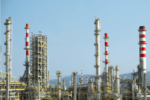
Source: Unsplash.com
The use of dynamic simulation will increase the adoption of novel designs and ultimately the efficiency of new or revamped plants. As these issues need to be analyzed in the early development of a process, the models will necessarily be simpler than the models used when the design has been completed. At this stage concepts are tested and one would not expect quantitative answers from a dynamic model but rather indications of process stability or control feasibility.
Safety Analysis
Much goes into ensuring that a plant will be safe for the operators and the people living in the neighborhood of the plant. Huge liabilities are associated with the safety of a plant. Some dynamic models are standard practice for any design, but surprisingly in other areas the use of dynamic models is still limited.
For virtually any plant operating at high pressure depressuring studies will be a standard part of the engineering phase. Depressuring studies are performed to analyze the behavior of pressure and temperature when the pressure of a plant that has been stopped is let down. The depressuring study defines the necessary flaring capacity that is needed and the results may also impact the choice of materials of vessels. Typically, if the pressure letdown of a vessel results in too low temperatures, carbon steel will have to be replaced with stainless steel to prevent the metal becoming too brittle. The other class of depressuring studies is related to the consequences of a fire in the area where a vessel is located. The main goal here is to determine the minimum vent rate that is needed to keep the vessel pressure under control and to bring down the vessel pressure to prevent a failure of the vessel wall as temperature rises.
Read also: The Resurgence of Liquefied Natural Gas in the Atlantic Basin and Qatar
All plants have emergency shutdown systems (ESD). The design of a system to safely stop the operation of part of or a complete plant can be very complex and it is often difficult to foresee all the consequences of everything that happens during a shutdown. A dynamic simulation model of the plant is an invaluable tool to set up an ESD system properly. Far too often it is seen that a dynamic model is used when an incident has taken place to analyze the exact causes of it when the use of such a model during the design phase might have prevented the occurrence of the incident all together.
Modeling the behavior of the plant under emergency shutdown conditions requires the model to be quite detailed and the simulation is usually more challenging than other applications. Under ESD conditions, much of the equipment is shut down, many flows are stopped, and any engineer knows that mathematics and zeros do not go very well together.
Start-Up Procedure Definition
Modeling the start-up procedure also requires a detailed model. Although generally the dry start condition also involves lots of stopped equipment and zero flows, it tends to be somewhat easier to model than an ESD scenario.
The use of a dynamic model to verify the start-up procedures of a plant can reduce the commissioning time by weeks. This exercise consists of adding the start-up logic to the model and to run this start-up logic while observing the behavior of the plant model. When problems occur, the model can be stopped and the start-up logic can be reviewed and rerun.
Not only does the start-up procedure become streamlined, the engineers that have worked on it acquire a detailed understanding of the behavior of the plant, which allows them to make better decisions during plant commissioning and subsequent operation of the plant.
Distributed Control System (DCS) Checkout
DCS checkout alone will not warrant the construction of a dynamic model of a plant, but if a model is available, the modifications needed to be able to run a DCS checkout are relatively small. The purpose of the DCS checkout is to verify that all the cabling connecting the DCS to the plant and the DCS internal TAG allocations are hooked up properly. Obviously a dynamic model will not be able to help with checking the physical cabling, but the signals from a dynamic model can replace the plant signals. This will help tremendously in verifying the logical connections inside the DCS. If a wrong measurement is routed to a particular controller, this will be seen quite readily as the dynamic model provides realistic numbers for these. It is much easier to discern an erroneous number among realistic numbers than to match quasi-random numbers.
Operator Training
A classical use of dynamic simulation has been for operator training systems. Nowadays this is just one of the applications that can be built on top of a detailed dynamic model. In most new projects an operator training system is becoming a standard requirement and it is yet another driver to start using dynamic simulation early in plant design, as part of the earlier work can be reused in an operator training system.
In addition to the dynamic model, operator training systems are composed of various other parts.
- The operator stations that mimic the real DCS operator stations or that serve as spare operator consoles.
- An instructor station to allow the instructor to monitor the student’s progress and to let him introduce a selection of failures or other problems the operator may encounter in the real plant.
- Possibly an automated system to assign a score to the performance of the operator and/or to let the operator run predefined training scenarios.
- Software and hardware for the communication between the various modules.
Advanced Process Control
Advanced process control, particularly multivariable predictive control (MPC), normally requires access to plant data and step test results from the operating plant. Hence, MPC is usually only implemented once the plant has been commissioned. With a dynamic model available, this is no longer a limitation and the necessary information can be obtained from the step tests on that model. This part is covered in more detail later.
Plant Operation
A dynamic model in Plant Operation and Maintenance of Hydrocarbon Containing Equipment and Processesplant operation will usually require justification on a single application. Although future uses of a dynamic model are certainly possible, these will usually not be considered to be a tangible reason or additional justification to create such a model. However, it is quite often easier to quantify the benefits that will be gained from the use of a dynamic model.
Troubleshooting
Issues in the control or operability of the plant can be resolved easier, safer, and with no loss of production using a dynamic model. A dynamic model can be exercised at will where the engineer has very little freedom to test things out on the real plant. Maintaining production on spec will almost always override the need for testing to solve a problem. The solution imagined by the plant engineer is not necessarily the right one and implementing an untested solution may lead to unsafe operation.
With a dynamic model, the worst that can happen is that the model fails. The engineer can test a large range of operating conditions to ensure that the implemented solution will hold up in abnormal conditions, for example.
Plant Performance Enhancement
Most plant engineers will accept it as a given that many of the controllers that are in a plant are operated in manual. This is frequently a source of added operating cost for the plant. A typical example would be the reflux rate of a distillation column that is set to a fixed relatively high value to ensure that the product is always meeting the specifications. Most of the time, say 85 % of the time, the reflux could be run significantly lower and only during less than 5 % of the time the fixed reflux is needed to maintain product quality. It is fairly easy to compute the financial benefit associated with keeping the controller in automatic.
The reason that controllers are put in manual is often related to the trust operators have in controllers. There are generally two possible reasons for distrust. Either the operator does not understand properly how the controller will cope with upsets or the controller has shown in the past that it is incapable of dealing with those upsets.
Even without a full operator training system, a dynamic model can be used to show the operators how a series of typical upsets will be handled by the control system. Some of the responses may appear illogical to the operators at first, and with a model the operator will not feel the pressure to act prematurely in order to ensure product quality. This can help instill more confidence in the automated control and let it run in automatic mode.
It will be interesting: Velocity Criteria for Sizing Multiphase Pipelines
Of course, the distrust of the operator may be well founded, but in this case the dynamic model can be used as described in Section “Troubleshooting” to improve the controller behavior and subsequently illustrate to the operator that the problem has been solved to restore trust.
Incident Analysis
Although this is by no means the best use of a dynamic model, it is all too often the first step toward using dynamic simulation. After an incident there is always the need to know why it happened. If the incident resulted in damages, there will be legal requirements to determine the root cause of the incident. A dynamic process simulation model will often be used in this analysis to determine the sequence of events on the process side that led up to the incident and how adequate the emergency shutdown procedures were to mitigate the consequences of the incident.
Operator Decision Support
Operator decision support is an emerging use of dynamic simulation models. In this type of application the dynamic simulation model is run in real time and is receiving the same input signals as the real plant. It is impossible to cover the entire plant with instrumentation to provide all the information one would like to obtain. The real-time model provides the operators and engineers with simulated measurements throughout the entire plant to better appreciate current operation. Typical parts of a plant that do not have all the instrumentation one would like are long pipelines and high temperature outlets of reactors or furnaces. A second use of the online model is its predictive capability. Assuming the dynamic simulation model is fast enough, it can be used to predict events minutes or even hours ahead of the actual event. This information can be used to improve the handling of the event and to keep the plant operating within specifications.
Operator Training
It is important for the operators to keep their knowledge of the plant operation up to date. Especially with highly automated plants it is important that operators are confronted with abnormal situations using the simulator.
New operators will also benefit from the use of an operator training system.
If is therefore very important to keep the operator training system that was installed as part of the plant commissioning up to date. This means that any change to the DCS screens and systems must also be made to the operator training system and that any change made to the plant must be made in the dynamic process model as well.
Advanced Process Control (APC)
Implementation of an advanced process control system requires a significant investment and such a decision is not taken lightly. A dynamic simulation model can assist in determining the relevance of an APC implementation and it can help streamline the implementation itself.
It is fairly straightforward to run the necessary step tests for the implementation of a multivariable predictive controller (MPC) on a dynamic process simulation. The results can be used to design the MPC and to run the MPC on the dynamic model. A comparison of the plant performance using the existing control system with the MPC can provide the necessary information to decide if an MPC implementation is an attractive investment. Running step tests on a model has a number of advantages over step tests on the real plant.
- No disturbance of the plant operation.
- Step tests can use a broader range of conditions.
- Step tests do not depend on the availability of plant personnel, plant incidents, and other events that are not compatible with step tests on the plant.
- The dynamic model does not suffer from valves that get stuck and other incidents that make life difficult when performing step tests.
- The dynamic model can be run faster than real time and hence step tests that would otherwise take days can be run in an hour or less.
When the final MPC controller has been designed and implemented, it can first be put online using the dynamic simulation model. This setup can be used to discover a significant part of the practical problems that would otherwise only surface during the commissioning of the MPC on the real plant. Although the MPC models should be verified for actual plant operation, this accelerates MPC commissioning and lowers the risk of production loss that may be experienced during commissioning of the MPC.
Modeling Considerations
Level of Detail in the Model
The level of detail required for a dynamic simulation model is very dependent on the application. Most of the time a model will contain components that are modeled in great detail (high fidelity) while other components only capture the overall dynamic behavior. A typical example is a model of a gas compressor.
An initial application is to use the model to analyze the behavior of the antisurge control logic. In this case it will be important to properly model all the gas volumes in the main gas lines and also in the antisurge system. The control logic used in the model will be an exact replication of the commercial system that will be installed. As compressor surge is a very fast phenomenon, these controllers have sampling times on the order of 50 milliseconds, the model will need to run using a time step that is capable of capturing these phenomena and hence have a time step that is even smaller than 50 milliseconds. As a consequence, the model may run slower than real time. However, as in this case, the time span of interest is a few minutes at the most, the slower model performance is not really a problem.
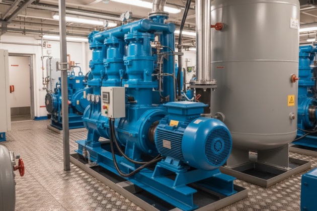
Source: AI generated image
A second application for this dynamic model of a compressor station may be for operator training. It is not relevant to model events that happen so fast that it is impossible for an operator to respond during the event.
On the one hand, the step size and hence the speed of the model can be increased. On the other hand, it will be important to include manually operated purge valves in the dynamic model to allow the operator to perform all actions he deems necessary. This is a bit of detail that is of no use for the initial application.
The level of detail required should be assessed based on the objectives for the model. This assessment is not a global assessment for the complete model, but the assessment should consider the objectives for each section of the plant down to each piece of equipment.
Model Speed
The speed of a model is expressed most frequently as the real-time factor of the model. This is the ratio of the simulated time divided by the real time. The speed requirements vary dependent on the application. For an operator training simulator, it is clear that the model needs to be capable of runoff running at least in real time (real time factor = 1). Quite often the real-time factor should be higher, up to 10 times real time. This allows the operator to fast forward through periods of stabilization of the process, for example.
Read also: Harnessing LNGC Longevity – Strategies for Sustainable Energy Transportation
For an engineering study, the important factor is the total amount of time it takes to study an event. Ideally, that time would be 10 minutes or less. This means that 3-hour events should have a real-time factor of 18 or higher. If the event to be studied only lasts for one minute, then a real time factor of 0,1 is acceptable.
The model speed is mainly affected by the following factors.
- Time step of the integrator.
- Complexity of the model.
- Number of components used to represent the fluids and the complexity of the thermodynamic model.
As the same factors will also affect the accuracy of the model, a balance must be found between speed and accuracy.
Equipment-Specific Considerations
The following sections recommend the information to consider when modeling various pieces of equipment. Depending on the available modeling tool, the recommended level of detail may differ. Recommendations only apply to the main aspects of the model.
Valves
The minimum requirement to model a valve properly is to use the correct Cv value and the type of The Selection and Testing of Valves for LNG Applicationsvalve characteristic. For some studies it is important to capture the dynamic behavior of the valve. For example, an emergency shutdown valve needs a certain time to close. For safety studies it is important to consider the time to close. Most plants will have one or more check valves. It is important to include these valves in the model, particularly when the model is used to run scenarios far away from normal operation.
Rotating Equipment
For pumps, compressors, and expanders, it is best to always use the performance curves of the equipment. If this information is not available, it is relatively simple to create a generic performance curve starting from the normal operating point of the equipment. This information is then complemented with either the speed or the absorbed power. For most motor-driven equipment, a speed specification will be the best option except when studying start-up and shutdown phenomena. For equipment driven by a gas turbine, a specification of the absorbed power is usually a better choice.
If the study concerns the start-up or shutdown of the equipment, it will be necessary to include details such as rotor inertia, friction losses, and dynamics of the driver (e. g., an electrical motor) in the model.
Piping Equipment
The level of detail for modeling the piping depends a lot on the application. For process piping, it is quite often sufficient to model the pressure loss. Most of the time the volume of the piping is negligible compared to the volume of the process equipment. A notable exception is the modeling of compressor antisurge systems. An accurate representation of the system volume is crucial in obtaining correct results. For transport pipelines the model should usually be more detailed, as the expected results may include information such as the time lag of a product in the pipeline, the evolution of the temperature, and the multiphase behavior of the fluid. The required information includes the pipeline elevation profile, the pipeline diameter, pipe schedule, insulation, and environment.
Columns
Distillation models should reflect the holdup volumes of both the liquid and the vapor phase properly. A significant difference between tray columns and packed columns is that the much smaller liquid holdup of packed columns will reduce the response time of the column compositional perturbations, for example.
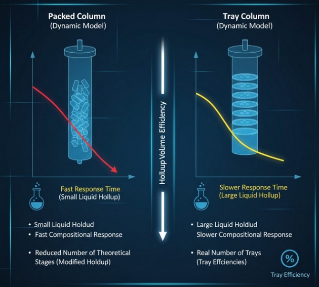
Source: AI generated image
It is customary to use a reduced number of theoretical stages to model distillation columns in steady-state simulations. If the same approach is used in a dynamic simulation, the tray or packing characteristics will be modified to use the correct holdup volumes for liquid and vapor. Another approach is to use tray efficiencies and keep the number of trays used equal to the number of real trays in the column. Keep in mind that the tray efficiency and the column overall efficiency are not the same.
Heat Exchangers
The level of detail for a heat exchanger will strongly depend on the role of the heat exchanger and the phenomena to be studied. For example, if the exchanger serves to cool down a condensate stream before it proceeds to storage and the focus of the study is on the equipment upstream of this exchanger, then it may be enough to use a model that simply assumes the exchanger is always cooling the fluid down to the required temperature. At the opposite side of the spectrum there would be a plate fin heat exchanger in a LNG Reliquefaction Plantnatural gas liquefaction plant. In this case the exchanger is the heart of the plant and the model needs to accurately represent the construction of the exchanger and to take into account elements such as the heat capacity of the metal and the dynamics of the metal temperature.
The model will need to provide information such as the temperature and pressure profiles inside the exchanger.
Control Systems
Contrary to steady-state simulation, the modeling of the control equipment is crucial to the success of a dynamic simulation model. Quite often the control strategy and controller tuning is the final objective of the dynamic simulation, but without proper configuration of the control system the model will quickly end up in totally abnormal operating conditions.
It will be interesting: Understanding Liquefied Gas Manifolds – Size Categories, Positioning, and Specific Designs for LPG & LNG
For regular proportional, integral, and derivative (PID) controllers, the main points to consider are correct direction of the action (reverse or direct) taken, realistic tuning constants, and proper span of the instrumentation. Once the simulation model has reached relatively stable conditions, attention can focus on a high-fidelity representation of the control systems.
The high-fidelity representation can come in various forms. For an operator training system, most of the DCS vendors will be able to provide software that emulates the DCS system. The model itself is then only used to represent the noncontrol equipment. The DCS emulation will receive the plant measurements from the model like the real DCS would receive the measurements from the plant and the DCS will send signals to the valve positioners according to the control algorithms defined in the DCS.
The verification of a surge controller for a compressor is also an area where a high-fidelity representation of the particular controller is crucial.
The representation can be built by combining blocks that are part of the dynamic simulator, by writing a custom model for the controller, by linking the model to an emulation program, or even linking the model to the controller hardware.
Control of Equipment and Process System
This section enumerates some typical applications of dynamic simulation in the various processes that are employed in Navigating Acid Gas Treating and Sulfur Reclamationgas treatment and transportation. The application is usually governed by the particular equipment used in the process.
Gas Gathering and Transportation
The key equipment in gas gathering and transportation are pipelines, valves, and compressors. The range of applications in this area is very wide.
- Assess the risk of condensate accumulation and associated slug sizes.
- Line packing capacity studies.
- Safety studies on pipeline shutdowns.
- Pipeline depressuring studies.
- Compressor station antisurge control studies.
Gas Treating
The main equipment used for the absorption of CO2 and H2S are absorption and regeneration columns using amine solutions to absorb the acid gas components. A dynamic model will prove useful if the quality of the feed gas can fluctuate significantly. In such a case, the product gas quality will be affected directly by the amount of amine solution that is circulated and also by the quality of the lean amine solution, which is influenced indirectly by the amount of acid gas in the feed.
Sulfur Recovery
The performance of a sulfur recovery unit is mainly governed by the operation of the various reactors in the process. A key factor in the reactor performance is the correct air-gas ratio of the reactor feed. If the acid gas feed is unstable, dynamic modeling can be used to select the best control strategy to cope with these fluctuations and to improve the controller tuning.
Gas Dehydration
The glycol Process and Operational Challenges in Natural Gas Dehydration Systems Join Our Telegram (Seaman Community)gas dehydration process is very similar to the acid gas removal process. Fluctuations in water content of the feed gas and gas flow rate affect the product gas quality. The control strategy ensures quality of the product by selecting the appropriate glycol flow rate and by maintaining the quality of the lean glycol.
Read also: LNG Developments – Key Milestones and Challenges in the Sector
For dehydration processes using mole sieve beds the application of dynamic simulation is similar to an application for plant start-up. The model would include the logic that is driving the bed switching and regeneration cycles. Once implemented in the model, the logic can be tested by running it on the model and by tracking critical operating parameters of the mole sieve unit.
Liquids Recovery, Natural Gas Liquefaction
A cold box is a key piece of equipment in these processes. The flows that exchange heat in the cold box exchanger create a multitude of thermal loops in the process, which make it more difficult to control. A detailed dynamic model of the overall process, including a detailed model of the cold box, will help understand the severity of the interactions created by these thermal loops. A control strategy designed to cope with these interactions can be tested thoroughly.
From the perspective of pressures and flows, the operation of turboexpanders or turboexpanders coupled to compressors is important. The efficiency of a turboexpander drops quickly as one deviates from the design conditions, and the impact of a temporary deviation of the operating conditions on the process dynamics is difficult to understand without help. A dynamic model will aid in understanding the behavior and in selecting the correct control structure and controller tuning to cope with a transient deviation from design conditions.
NGL Fractionation
NGL fractionation is composed of a series of distillation columns. As the purity specs on the columns are fairly severe on both the top and the bottom products, the control of the columns is not straightforward.
A dynamic model will provide the capability to select the best control strategy given the particular column operation and specifications and given the expected disturbances in the feeds.
Case Study I: Analysis of a Fuel Gas System Start-up
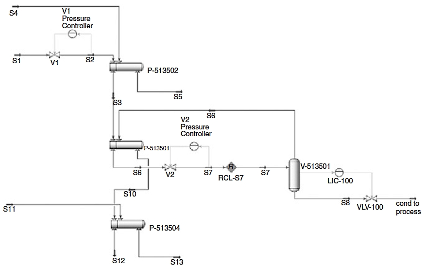
This study analyzes the start-up philosophy of the fuel gas system of a Latin American offshore platform. The fuel gas system PID is shown in Figure 1.
It is thought from steady-state analysis that the system can be started up using cold pipeline gas without preheating.
Introduction
Under normal operation the fuel gas burnt in turbogenerators (TGs) comes from the platform main compression system at 180 kg/cm2 and 38 °C. At the system inlet, the pressure is reduced to 100 kg/cm2 and the temperature goes down to 17 °C. The fuel gas is then preheated in P-513502 to 60 °C with hot water and another pressure reduction to 45 kg/cm2 through a Joule-Thompson (JT) valve, resulting in a temperature of around 16 °C.
After this last pressure reduction, the mixture of condensate and gas is sent to a condensate vessel drum (V-513501), the condensate returns to the process, and the gas from the vessel proceeds through a gas-gas heater exchanger (P-513501). This LNG (Liquefied Natural Gas) as Fuelfuel gas from P-513501 at an average temperature of 43 °C is reheated with hot water in heat exchanger P-513504 to around 63 °C and is sent to the turbo generators.
It will be interesting: Key Aspects and Recommendations for the Safety Zone for LNG Bunkering
The objective of the system is to produce a fuel gas stream with a defined rate, a defined pressure, and a temperature at least 20 °C above the dew point. This is a minimum value demanded by the turbogenerator vendor. The fuel gas exit temperature must also be maintained above 0 °C to meet material temperature limitations.
During the start-up/restart of the platform there is no Mastering Natural Gas Fundamentals Properties Sources and Transport Insightsgas source on the platform but cold pipeline gas can be imported at 5 °C. Also, there is no hot water available for the preheaters. One solution is to start the turbogenerators with diesel. This solution is undesirable, as diesel needs to be imported onto the platform, the turbogenerators need to be adapted to cope with diesel feed, and several other problems lead to production inefficiency and unnecessary cost.
The objective of the dynamic simulation is to study the exact behavior of the fuel gas system under the start-up condition of cold pipeline import gas and the circulation of the sea water at 25 °C to heat the gas.
Steady-State Analysis
The steady-state results clearly show that thermodynamically and theoretically both normal operating and cold start scenarios result in gas feeds to the turbo generators that are well above the dew point approach limitation of 20 °C. Hence it seems feasible to provide fuel gas with a temperature at 20 °C above dew point. However, this does not account for the transients encountered during startup. The question can only be answered conclusively by a dynamic analysis.
Dynamic Analysis
In the first start-up scenario water is circulating at 25 °C before any gas is fed. Once the water flow is stable, cold pipeline gas is brought on stream. The strip charts from a HYSYS dynamics model displaying the system temperatures for this case are shown in Figure 2.
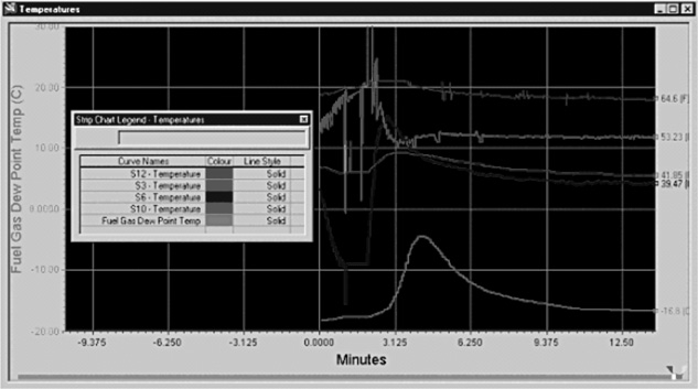
As the cold import gas hits the warmer exchangers the gas is heated and some of the heavier components flash off in the condensate drum and pass back through the gas-gas chiller. The dew point of the fuel gas then rises for about 4 minutes until eventually the chill duty in the recycle and the JT effect in valve V2 stabilize. The temperature of the fuel gas outlet remains relatively constant as the heat exchange in P-513504 is established. Hence there is a closer approach between the fuel gas temperature and the dew point, reaching 24 °C at 4,1 minutes. This is too close to the limit to accept without further study.
The second start-up scenario assumes that the cold pipeline gas flow is established first and that the Complete Guide to Below Deck Sailboat Systemswater system is brought on line afterward.
The strip charts of the system temperatures in this case are shown in Figure 3.
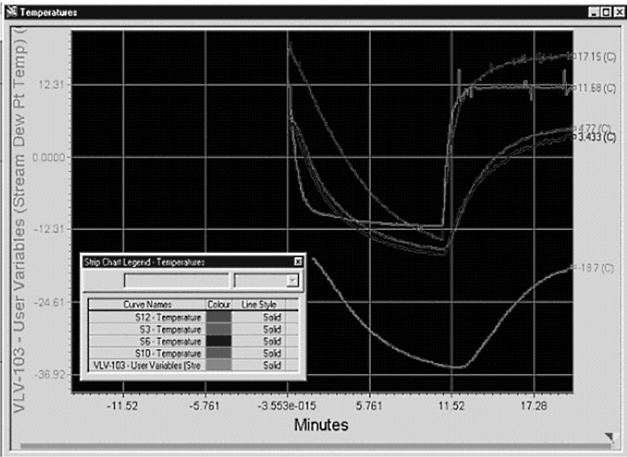
Because the JT effect and cold duty on the gas-to-gas exchanger, the gas dew point does not initially increase but maintains a difference from stream 12 temperature. In this mode they would eventually equate. Also the fuel gas exit temperature is decreasing and within 4 minutes it will reach the material temperature limit of 0 °C. On start up of the water system the temperature recovers after 10 minutes and the fuel gas always maintains more than a 40 °C difference from the dew point.
Conclusion
A dynamic model clearly shows potential problems with all start-up modes of the platform fuel gas system with minimum approaches to dew point or minimum material temperatures. However, the dynamic model also demonstrates a combination of procedures, starting with the water off and then increasing flow quickly, that could maintain all proper flow rates and temperatures for fuel gas start up without diesel, thus saving millions of dollars.
Case Study II: Online Dynamic Model of a Trunk Pipeline
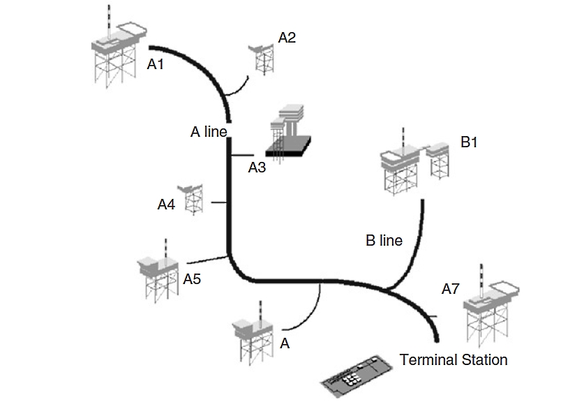
The 235-mile NOGAT trunk line is located in the Dutch part of the North Sea, and it connects eight offshore platforms to onshore gas processing facilities near Den Helder, The Netherlands. Each platform delivers both gas and condensate to the pipeline so the line operates inside the two-phase region; two of the platforms sit on oil fields and the off gas from the oil stabilization units is compressed and delivered to the pipeline. The current total capacity of the Harnessing LNGC Longevity – Strategies for Sustainable Energy Transportationgas transportation system is about 22 million m3/day, associated with 750 m3 of condensate/day.
Read also: Navigating Acid Gas Treating and Sulfur Reclamation
The onshore facilities include a 1 000-m3 slug catcher, condensate stabilization units that remove volatile components from the trunk line produced liquids, and a series of low-temperature separation (LTS) units to dry the sales gas prior to delivery to the distribution network.
Figure 4 shows a representation of the system.
There are two major challenges to operating the system.
- Controlling the sales gas quality in terms of its Wobbe index. The Wobbe index is a measure used to compare the equivalent thermal content characteristics of different gases. It is defined as a volumetric high heating value divided by the square root of relative density to air.x The different platforms produce different gas qualities and quantities that are fed into the line at different locations. Therefore, the quality of the gas that travels through the trunk line varies along its length and also with time. Despite this, the sales gas quality must stay within the contractual limits at all times (i. e., Wobbe index values between 49 and 54).
- Controlling the condensate inventory of the trunk line. The amount of condensate retained inside the line builds up during periods of low gas demand, particularly in trunk line depressions. The available slug catchers and condensate stabilization unit capacities limit the production ramp-up speed and force the scheduling of periodic cleanup cycles to keep the trunk line liquid holdup below certain critical limits.
This chapter discusses the elements of automating today’s Natural Gas Processing and Liquids Recoverygas processing plants, including considerations for instrumentation, controls, data collection, operator information, optimization, and management information. The advantages and disadvantages of various approaches are analyzed in this chapter. Also, strategies for identifying and quantifying the benefits of automation are discussed.

- Brown, C., and Hyde, A., “Dynamic Simulation on the Shell Malampaya Onshore Gas Plant Project”. Paper presented at the GPA Europe Annual Conference, Rome, Italy (Sept. 25-27, 2001).
- La Riviére, R., and Rodriguez, J-C., “Program tracks wet-gas feedstocks through two-phase offshore trunkline”. Oil Gas J. 103(14), 54-59 (2005).
- Valappil, J., Messersmith, D., and Mehrotra, V., LNG lifecycle simulation. Hydrocarb. Eng. 10, 10 (2005).
- Wassenhove, W. V., Analysis of fuel gas system startup with HYSYS dynamic process simulation. Oil Asia J. 18-20 (January-March 2003).
- Young, B., Baker, J., Monnery, W., and Svrcek, W. Y., Dynamic simulation improves gas plant SRU control-scheme selection. Oil Gas J. 99, 22 (2001).