Effective Sales Gas Transmission is the crucial link in the energy supply chain, ensuring safe and reliable long-distance delivery of processed natural gas to end-users. This article delves into the core engineering principles governing pipeline design and operation. We will systematically explore flow fundamentals, friction factor correlations, and transient analysis, alongside the essential components of the gas network, including compressor stations and their various configurations.
- Gas Flow Fundamentals
- General Flow Equation
- Friction Factor Correlations
- Practical Flow Equations
- Predicting Gas Temperature Profile
- Transient Flow in Gas Transmission Pipelines
- Compressor Stations and Associated Pipeline Installations
- Compressor Drivers
- Compressors Configurations
- Reduction and Metering Stations
- Design Considerations of Sales Gas Pipelines
- Line Sizing Criteria
- Compressor Station Spacing
- Compression Power
- Pilpeline Operations
Natural gas continues to play a great role as a worldwide energy supply. In fact, major projects are being planned to move massive amounts of high-pressure sales gas from Natural Gas Processing and Liquids Recoveryprocessing plants to distribution systems and large industrial users through large-diameter buried pipelines. These pipelines utilize a series of compressor stations along the pipeline to move the gas over long distances. In addition, gas coolers are used on the discharge side of the compressor stations to maintain a specified temperature of the compressed gas for pipeline downstream pressure drop reduction and to protect gas pipeline internal and external coating against deterioration due to high temperatures. This chapter covers all the important concepts of sales gas transmission from a fundamental perspective.
Gas Flow Fundamentals
Optimum design of a gas transmission pipeline requires accurate methods for predicting pressure drop for a given flow rate or predicting flow rate for a specified pressure drop in conjunction with installed compression power and energy requirements, e. g., fuel gas, as part of a technical and economic evaluation. In other words, there is a need for practical methods to relate the flow of gas through a pipeline to the properties of both the pipeline and gas and to the operating conditions, such as pressure and temperature. Isothermal steady-state pressure drop or flow rate calculation methods for single-phase dry Pipelines in Marine Terminals: Key Considerations for Handling Liquefied Gasgas pipelines are the most widely used and the most basic relationships in the engineering of gas delivery systems. They also form the basis of other more complex transient flow calculations and network designs.
General Flow Equation
Based on the assumptions that there is no elevation change in the pipeline and that the condition of flow is isothermal, the integrated Bernoulli’s equation is expressed by Equation 1:
where:
- Qsc – is standard gas flow rate, measured at base temperature and pressure, ft3/day;
- Tb – is gas temperature, base conditions, 519,6 °R;
- Pb – is gas pressure, base conditions, 14,7 psia;
- P1 – is inlet gas pressure, psia;
- P2 – is outlet gas pressure, psia;
- D – is inside diameter of pipe, inches;
- f – is Moody friction factor;
- E – is flow efficiency factor;
- γG – is gas specific gravity;
- Ta – is average absolute temperature of pipeline, °R;
- Za – is average compressibility factor;
- L – is pipe length, miles;
- and C – is 77,54 (a constant for the specific units used).
Although the assumptions used to develop Equation 1 are usually satisfactory for a long pipeline, the equation contains an efficiency factor, E, to correct for these assumptions. Most experts recommend using efficiency factor values close to unity when dry gas flows through a new pipeline. However, as the pipeline ages and is subjected to varying degrees of corrosion, this factor will decrease. In practice, and even for single-phase gas flow, some water or condensate may be present if the necessary drying procedure for gas pipeline commissioning is not adopted or scrubbers are not installed. This puts compression equipment at risk of damage and also allows localized corrosion due to water spots (wetting of the pipe surface). The presence of liquid products in the Raw Gas Transmission: Multiphase Flow, Hydrates, and Corrosion Challengesgas transmission lines can also cause drastic reduction in the flow efficiency factor. Typically, efficiency factors may vary between 0,6 and 0,92 depending on the liquid contents of the pipeline.
Read also: LNG Panel Erection and Sealing Techniques
As the amount of liquid content in the gas phase increases, the pipeline efficiency factor can no longer account for the two-phase flow behavior and two-phase flow equations must be used.
Pipelines are usually not horizontal; however, as long as the slope is not too great, a correction for the static head of fluid (Hc) may be incorporated into Equation 1 as follows.
where:
and
- H1 – is inlet elevation, ft;
- H2 – is outlet elevation, ft;
- and g – is gravitational constant, ft/sec2.
The average compressibility factor, Za, is determined from the average pressure (Pa) and average temperature (Ta), where Pa is calculated from Equation 4:
where:
- P1 and P2 are the upstream and downstream absolute pressures, respectively.
The average temperature is determined by Equation 5.
In the Equation 5, parameter TS is the soil temperature, and T1 and T2 are the upstream and downstream temperatures, respectively.
Having obtained Pa and Ta for the gas, the average compressibility factor can be obtained using Kay’s rule and gas compressibility factor charts.
Friction Factor Correlations
The fundamental flow equation for calculating pressure drop requires a numerical value for the friction factor. However, because the friction factor, f, is a function of flow rate, the whole flow equation becomes implicit. To determine the friction factor, fluid flow is characterized by a dimensionless value known as the Reynolds number [Equation 6].
where:
- NRe – is Reynolds number, dimensionless;
- D – is pipe diameter, ft;
- V – is fluid velocity, ft/sec;
- ρ – is fluid density, lbm/ft3;
- and µ – is fluid viscosity, lbm/ft.sec.
For Reynolds numbers less than 2000 the flow is considered laminar. When the Reynolds number exceeds 2000, the flow is characterized as turbulent. Note that in high-pressure gas transmission pipelines with moderate to high flow rates, only two types of flow regimes are observed: partially turbulent flow (smooth pipe flow) and fully turbulent flow (rough pipe flow). For gases, the Reynolds number is given by Equation 7.
where:
- D – is pipe diameter, inches;
- Qsc – is gas flow rate, standard ft3/day;
- µG – is gas viscosity, cp;
- Pb – is base pressure, psia;
- Tb – is base temperature, °R;
- and γG – is gas specific gravity, dimensionless.
For the gas industry, Equation 7 is a more convenient way to express the Reynolds number, as it displays the value proportionally in terms of the gas flow rate.
The other parameter in the friction factor correlation is pipe roughness (ε), which is often correlated as a function of the Reynolds number and the pipe relative roughness (absolute roughness divided by inside diameter). Pipe roughness varies considerably from pipe to pipe, and Table 1 shows the roughness for various types of new (clean) pipes.
| Table 1. Pipe Roughness Value | |
|---|---|
| Type of pipe (new, clean condition) | ε (inches) |
| Carbon steel corroded | 0,019685 |
| Carbon steel noncorroded | 0,001968 |
| Glass fiber reinforced pipe | 0,0007874 |
| Steel internally coated with epoxy | 0,00018 to 0,00035 |
These values should be increased by a factor ranging between 2 and 4 to account for age and use.
The Moody friction factor, f, in Equation 1 is determined from the Moody diagram. The Moody correlation is shown in Figure 1. The Moody diagram consists of four zones:
- laminar,
- transition,
- partially turbulent,
- and fully turbulent zones.
The laminar zone, the left side, is the zone of extremely low flow rate in which the fluid flows strictly in one direction and the friction factor shows a sharp dependency on flow rate.
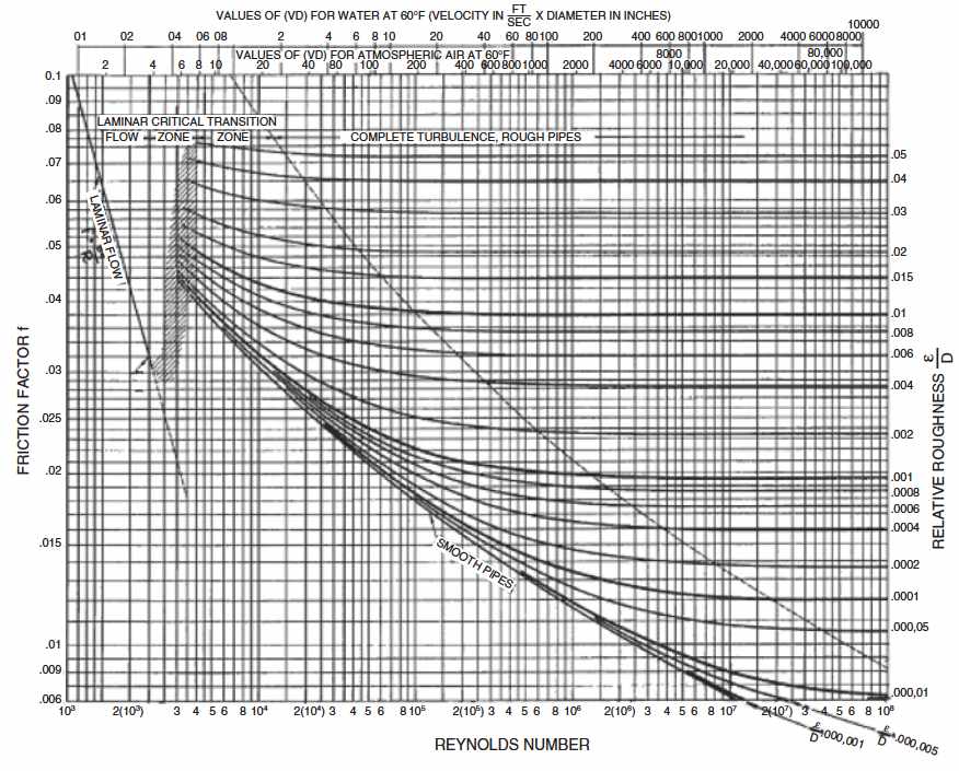
The friction factor in the laminar regime is defined by the Hagen-Poiseuille equation.
The fully turbulent zone, the right side, describes fluid flow that is completely turbulent (back mixing) laterally as well as in the primary direction.
The turbulent friction factor shows no dependency on flow rate and is only a function of pipe roughness, as an ideally smooth pipe never really exists in this zone. The friction factor to use is given by the rough pipe law of Nikuradse [Equation 9].
Equation 9 shows that if the roughness of the pipeline is increased, the friction factor increases and results in higher pressure drops. Conversely, by decreasing the pipe roughness, lower friction factor or lower pressure drops are obtained. Note that most pipes cannot be considered ideally smooth at high Reynolds numbers; therefore, the investigations of Nikuradse on flow through rough pipes has been of significant interest to engineers.
The partially turbulent (transition) zone is the zone of moderately high flow rate in which the fluid flows laterally within the pipe as well as in the primary direction, although some laminar boundary layer outside the zone of roughness still exists. Partially turbulent flow is governed by the smooth pipe law of Karman and Prandtl:
This correlation has received wide acceptance as a true representative of experimental results. However, a study by Zagarola on the flow at high Reynolds numbers in smooth pipes showed that the relevant correlation was not accurate for high Reynolds numbers, where the correlation was shown to predict too low values of the friction factor.
Consensus on how the friction factor varies across the transition region from an ideal smooth pipe to a rough pipe has not been reached. However, Colebrook presented additional experimental results and developed a correlation for the friction factor valid in the transition region between smooth and rough flow. The correlation is as follows:
This equation is universally accepted as standard for computing friction factor of rough pipes. Moody concluded that the Colebrook equation was adequate for friction factor calculations for any Reynolds number greater than 2000. Certainly the accuracy of the equation was well within the experimental error (about ±5 % for smooth pipes and ±10 % for rough pipes). However, the transcendental nature of the Colebrook equation is not conducive to simulation codes, as iteration is required.
It will be interesting: Comprehensive Overview of LNG Risk Management
In addition, this equation is problematic to program, as convergence is dependent on a reasonable initial guess for the friction factor. This is not insurmountable, of course, but the complication should be avoided if possible. It is recommended that the modified Colebrook equation be used in practical engineering calculations for pipe flow in place of the classical equation at no loss and significant gain. Garland et al. provide additional details on this subject. Note that an explicit correlation for friction factor was presented by Jain. This correlation is comparable to the Colebrook correlation and does not require iteration. For relative roughness between 0,000001 and 0,01 and the Reynolds number between 5 × 10³ and 1 × 10⁸, the errors were within 1 % when compared with the Colebrook correlation. Therefore, it is usually recommended for all calculations requiring friction factor determination of turbulent flow.
The friction factor is sometimes expressed in terms of the Fanning friction factor, which is one-fourth of the Moody friction factor. Care should be taken to avoid inadvertent use of the wrong friction factor.
Practical Flow Equations
The Moody friction factor, f, is an integral part of the general gas flow equation. Because it is a highly nonlinear function, it must be either read from a chart or determined iteratively from a nonlinear equation. Approximations to the Moody friction factor have been widely used because they allow the gas flow equation to be solved directly instead of iteratively. The four most widely published friction factor approximations are Weymouth, Panhandle A, Panhandle B, and IGT. The Weymouth equation approximates the Moody friction factor by Equation 12, and the remaining three equations approximate the friction factor by Equation 13, where “m” and “n” are constants.
These constants are given in Table 2.
| Table 2. Constants in Equations 12 and 13 | ||
|---|---|---|
| Equation | m | n |
| Weymouth | 0,032 | 0,333 |
| Panhandle A | 0,085 | 0,147 |
| Panhandle B | 0,015 | 0,039 |
| IGT | 0,187 | 0,200 |
The Reynolds number, NRe, can be approximated by Equation 7. In addition to the Reynolds number, the pipe roughness also affects the friction factor for turbulent flow in rough pipes. Hence, the efficiency factor is chosen to correctly account for pipe roughness.
These approximations can then be substituted into the flow equation for f, and the resulting equation is given by Equation 14.
In Equation 14 the values for a1 through a5 are constants that are functions of the friction factor approximations and the gas flow equation.
These constants are given in Table 3.
| Table 3. Constants in Equation | |||||
|---|---|---|---|---|---|
| Equation | a1 | a2 | a3 | a4 | a5 |
| Weymouth | 433,46 | 2,667 | 0,5000 | 0,5000 | 0,000 |
| Panhandle A | 403,09 | 2,619 | 0,4603 | 0,5397 | 0,0793 |
| Panhandle B | 715,35 | 2,530 | 0,4900 | 0,5100 | 0,0200 |
| IGT | 307,26 | 2,667 | 0,4444 | 0,5556 | 0,1111 |
Inspection of Table 3 shows that the gas flow rate is not a strong function of the gas viscosity at high Reynolds numbers because viscosity is of importance in laminar flow, and gas pipelines are normally operated in the partially/fully turbulent flow region. However, under normal conditions, the viscosity term has little effect because a 30 % change in absolute value of the viscosity will result in only approximately a 2,7 % change in the computed quantity of gas flowing. Thus, once the gas viscosity is determined for an operating pipeline, small variations from the conditions under which it was determined will have little effect on the flow predicted by Equation 14.
Note that all of the equations noted earlier have been developed from the fundamental gas flow equation; however, each has a special approximation of the friction factor to allow for an analytical solution. For instance, the Weymouth equation uses a straight line for f, and thus, its approximation has been shown to be a poor estimation for the friction factor for most flow conditions. This equation tends to overpredict the pressure drop, and thus provides a poor estimate relative to the other gas flow equations. The Weymouth equation, however, is of use in designing gas distribution systems in that there is an inherent safety in over predicting pressure drop. In practice, the Panhandle equations are commonly used for large-diameter, long pipelines where the Reynolds number is on the flat portion of the Moody diagram. The Panhandle “A” equation is most applicable for medium to relatively large diameter pipelines (12″ – 60″ diameter) with moderate gas flow rate, operating under medium to high pressure (800 – 1 500 psia). The Panhandle “B” equation is normally appropriate for high flow rate, large-diameter (< 36″), and high-pressure (< 1 000 psi) transmission pipelines.
Because friction factors vary over a wide range of Reynolds number and pipe roughness, none of the gas flow equations is universally applicable.
However, in most cases, pipeline operators customize the flow equations to their particular pipelines by taking measurements of flow, pressure, and temperature and back calculating pipeline efficiency or an effective pipe roughness.
Predicting Gas Temperature Profile
Predicting the pipeline temperature profile has become increasingly important in both the design and the operation of pipelines and related facilities. Flowing gas temperature at any point in a pipeline may be calculated from known data in order to determine:
- location of line heaters for hydrate prevention;
- inlet gas temperature at each compressor station;
- and minimum gas flow rate required.
to maintain a specific gas temperature at a downstream point. To predict the temperature profile and to calculate pressure drop accurately, it is necessary to divide the pipeline into smaller segments. The temperature change calculations are iterative, as the temperature (and pressure) at each point must be known to calculate the energy balance. Similarly, the pressure loss calculations are iterative, as the pressure (and temperature) at each point along the pipeline must be known in order to determine the Chemical Composition and Physical Properties of Liquefied Gasesphase physical properties from which the pressure drop is calculated.
It will be interesting: LNG Bunkering Hazardous Zone: Safety, Classification, and Control
Thus, generating a usable temperature profile requires a series of complex, interactive type calculations for which even the amount of data available in most cases is insufficient. Additionally, the pipeline outer environment properties such as soil data and temperatures vary along the pipeline route and therefore play a very important role and require a consistent modeling to provide a reliable temperature profile evaluation. A simple and reasonable approach is to divide the pipeline into sections with defined soil characteristics and prevailing soil temperatures for summer and winter time and then to calculate the overall heat transfer that will be highly influenced by the outer conditions. The complexity of this method has led to the development of approximate analytical methods for the prediction of temperature profile, which in most situations are satisfactory for engineering applications.
Basic relationships needed for these calculation methods are thermal, mechanical energy balances, and mass balance for the gas flow in pipelines. The general or thermal energy balance can be written as follows.
where:
- T – is gas temperature;
- P – is absolute pressure of gas;
- V – is gas linear velocity in the pipeline;
- q – is heat loss per unit mass of flowing fluid;
- Cp – is constant pressure-specific heat;
- η – is Joule-Thomson coefficient;
- H – is height above datum;
- x – is distance along pipeline;
- gc – is conversion factor;
- and g – is gravitational acceleration.
The major assumption in the development of Equation 15 is that the work term is zero between the Reciprocating and Centrifugal Compressor Comparison for Natural Gas Compressioncompressor stations.
To calculate heat transfer from the pipe to the ground (soil), per unit of pipeline length, the Kennelly equation, Equation 16, is used:
where:
- K – is thermal conductivity of soil;
- TS – is undisturbed soil temperature at pipe centerline depth;
- mG – is mass flow rate of gas;
- H′ – is depth of burial of pipe (to centerline);
- and D0 – is outside diameter of pipe.
A basic assumption in Equation 16 is that the temperature of the gas is the same as the temperature of the pipe wall (the resistances to heat transfer in the fluid film and pipe wall are negligible).
The mechanical energy balance is given by Equation 17.
where:
- ρ – is density of gas;
- f – is Fanning friction factor;
- and Di – is inside diameter of pipe.
The continuity equation, Equation 18, relates velocity to the pressure and temperature:
where:
- A – is inside cross-sectional area of pipe;
- and Z – is gas compressibility factor.
Equations 15 to 18 are the basic equations that must be solved simultaneously for calculation of the gas temperature and pressure profiles in pipelines. Details for solving this set of equations can be found in textbooks on numerical analysis, such as Constantinides and Mostoufi.
The typical equations used to determine pipeline temperature loss are the integrated form of the general equations. However, assumptions and simplifications must be made to obtain the integrated equations, even though the effects of these assumptions or simplifications are not always known. A major advantage of numerical integration of the differential equation is that fewer assumptions are necessary.
Considering this fact, Coulter and Bardon have presented an integrated equation as follows:
where:
- T1 – is the inlet gas temperature and the term “a” is defined as:
where:
- R – is pipe radius;
- and U – is overall heat transfer coefficient.
Equation 19 can be used to determine the temperature distribution along the pipeline, neglecting kinetic and potential energy and assuming that heat capacity at constant pressure, CP, and the Joule-Thomson coefficient remain constant along the pipeline. For most practical purposes, these assumptions are close to reality and generally do give quite good results. Moreover, for a long gas transmission pipeline with a moderate to small pressure drop, the temperature drop due to expansion is small and Equation 19 simplifies to Equation 21:
Equation 21 does not account for the Joule-Thomson effect, which describes the cooling of an expanding gas in a transmission pipeline. Hence, it is expected that the fluid in the pipeline will reach soil temperature later than that predicted by Equation 19.
Read also: Interbarrier Space Protection: Pressurization, Inertization and Scaffolding Techniques
While there has been extensive effort in the development of such pipelines, little attention has been paid to the fact that the Joule-Thomson coefficient and heat capacity at constant pressure are not constants.
However, a new analytical technique for the prediction of temperature profile of buried gas pipelines has been developed by Edalat and Mansoori, while considering the fact that η and CP are functions of both temperature and pressure. Readers are referred to the original reference for a detailed treatment of this method.
Example 1
A 0,827 specific gravity gas flowing at 180 MMscfd is transferred through a 104,4-mile horizontal pipeline with a 19-inch internal diameter. The inlet pressure and temperature are 1 165 psia and 95 °F, respectively. The desired exiting pressure is 735 psia. Assuming an overall heat transfer coefficient of 0,25 Btu/hr.ft2.°F, Joule-Thomson coefficient of 0,1093 °F/psi, gas heat capacity (CP) of 0,56 Btu/lbm°F, and soil temperature of 60 °F, how far will the gas travel before its temperature reaches the hydrate formation temperature? (Note that these conditions are very rare, as all export gas is dried to avoid hydrates. Hydrates could form in an export gas pipeline only when the dehydration unit breaks or the inhibitor pump breaks.)
Solution
Using the given data:
Solving Equation 19 gives:
By simultaneously using the just-described equation and the Velocity Criteria for Sizing Multiphase PipelinesKatz gravity chart, for prediction of hydrate formation temperature, the location of hydrate formation is determined. In this case, the hydrate formation temperature is 70,5 °F. The first location where hydrate formation occurs is 24,94 miles along the pipeline. However, Equation 21 is often used for most practical gas transmission pipelines. Using the solution with these parameters becomes
Based on this equation, the first location of hydrate formation is 48,62 miles along the line, which means Equation 21 predicts that the fluid in the pipeline will form hydrate much later than that predicted by Equation 19.
It should be noted that in this example the temperature profile is strongly affected by both the heat transfer coefficient, U, and the Joule-Thomson coefficient, η. According to Equation 19, heating would be required from 24,94 miles until 104,4 miles to prevent hydrate formation. This result depends strongly on U, η, and the soil temperature TS. If the pipe was insulated more strongly and U was reduced to 0,1 Btu/hr.ft2, the point where line heating is required would be extended out to 36,67 miles but heating would still be required. It is also of note that the outlet temperature would drop to 45,87 °F when U = 0,25 Btu/hr.ft2.°F and to 43,27 °F when U = 0,1 Btu/hr.ft2.°F, both of which are below the outside soil temperature. This result may seem surprising to the reader but it occurs due to the large pressure drop in the pipeline. In this case, line insulation is exacerbating the problem because it does not allow the soil to retard the Joule-Thompson cooling effect. Equation 21 is not able to account for this effect at all.
It will be interesting: Navigating the Complexities of an LNG Bunkering Permit
In order to prevent the formation of hydrates, the temperature must be such that no point in the pipeline is in the region where a hydrate will form.
A common technique to avoid hydrate formation in onshore gas transmission pipelines is thermal stimulation. Thermal stimulation involves the use of a source of heat applied directly in the form of injected steam or hot liquids or indirectly via electric means. The addition of heat raises the temperature of the pipeline and forces hydrates to decompose. The direct approach works well during steadytate conditions but is of no benefit in certain transient or shut-in scenarios. However, indirect heat, such as the installation of line heaters for onshore gas transmission systems, is feasible for these transient conditions. This technology is particularly applicable to transmission and distribution systems that operate in cold climates. The other method to avoid/prevent hydrate formation is insulation. In fact, the proper use of insulation may, in some case, negate the requirement for a heater altogether.
Transient Flow in Gas Transmission Pipelines
Pipeline operation is such that transmission pipeline gas flow exists in the unsteady state, primarily due to variations in demand, inlet and outlet flows change, compressor start and stop, control setpoints, etc. In fact, steady-state operation is a rarity in practice. The unsteady nature of the gas flow indicates the need for a useful transient flow pipeline model to represent such conditions. In other words, the model should solve time-dependent flow equations. When modeling lines, however, it is sometimes convenient to make the simplifying assumption that flow is isothermal and steady state as long as we incorporate a load or swing factor contingent to a latter transient design checking to prevent inadequate pipeline sizing. The steady-state models are widely used to design pipelines and to estimate the flow and line pack. However, there are many situations where an assumption of steady-state flow and its attendant ramifications produce unacceptable engineering results. Unsteady state flow of gas in transmission lines can be described by a one-dimensional approach and by using an equation of state, continuity equation, momentum, and energy equations. In practice, the form of the mathematical relationships depends on the assumptions made based on the operating conditions of the pipelines.
For the case of slow transient flows due to fluctuations in demand, it is assumed that the gas in the line has sufficient time to reach thermal equilibrium with its constant temperature surroundings. Similarly, for the case of rapid transient flows, it is assumed that the pressure changes occur instantaneously, allowing no time for heat transfer between the gas in the pipeline and the surroundings. However, for this case, heat conduction effects cannot be neglected. Streeter and Wylie have presented different methods that provide an accurate means of simulating unsteady state flow in gas transmission lines. For a detailed description of these method variations, which are beyond the scope of present discussion, readers are referred to the original paper.
Compressor Stations and Associated Pipeline Installations
Compressor stations are installed along the pipeline to boost the gas pressure in the pipeline to increase the pipeline capacity in order to meet the gas demand made by the users. Compressor stations comprise one or more compressor units, each of which will include a compressor and driver together with valves, control systems and exhaust ducts and noise attenuation systems. Each compressor station will have inlet filters or knock out vessels to protect the compressors from damage due to liquids and entrained particles. In addition to compressor stations, there may be gas injection and delivery points along the line where the pressure and flow will have to be monitored and controlled. Each of these locations will include pressure control facilities and flow measurement.
Compressor Drivers
Transmission systems have high volume flow and the compressor stations generally have low head. Centrifugal compressors are ideal for these low-head and high-volume applications. Centrifugal compressors are also high-speed machines and ideally should have high-speed drivers. Choices for drivers can be gas turbines, gas engines, and electric motors.
The selection is usually based on considerations of cost, both capital and maintenance, fuel or energy cost, reliability, and availability. Dealing with each of these in turn, gas engines are low speed and therefore will require a gearbox to connect to the compressor. Gas engines are really not competitive with other drivers in terms of installed cost at the power levels demanded by large-diameter, high-pressure pipeline transmission systems.
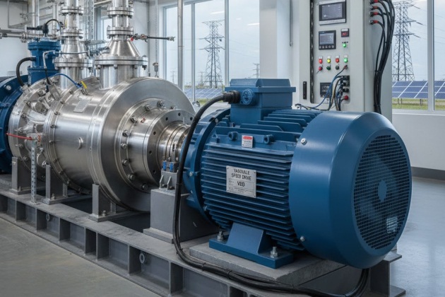
Source: Pixabay.com
Gas turbines are high-speed machines and can be directly coupled to the compressor and of course are available speed drives. Self-Survey Criteria for the Engine and Electrical SystemsElectric motors can be of several types with both fixed and variable speed options. Variable speed drivers (VSD) with electric motors present an overall performance much better than gas turbines and their selection depends on the site logistics and availability of electric energy at a reasonable price. They are very competitive in installed cost with comparable gas turbines. VSDs offer very low maintenance costs, rapid starting, lower noise levels, and no CO2 emission.
The decision to use gas turbine or electric motor drivers is almost always based on the site logistics, cost, availability, and reliability of the energy source. There will always be gas in the pipeline so the question of reliability and availability of the energy source for the gas turbine does not enter into the question. For the electric drive, there has to be a reliable electric grid within a short distance from the compressor station, transmission lines are costly, and there should be a backup independent feed to guard against line failure. Given that these conditions are satisfied, the decision then comes down to a matter of fuel versus electricity cost, overall performance, maintenance, and operation cost, which is usually demonstrated with a life cycle cost calculation and economic evaluation. The life cycle cost must examine and test the results for sensitivity to cost escalation in power prices and Understanding the Fundamentals of US Natural Gas Pricing and Market Volatilitygas price, taking into account the correlation between these two commodities.
Read also: New and Emerging LNG/CNG Markets
A long-term power supply agreement would be required to mitigate risk. The question of using a diesel engine as a power source as not been considered as it offers no advantages over a similar gas engine and it introduces another fuel, which invokes additional costs for transportation and storage.
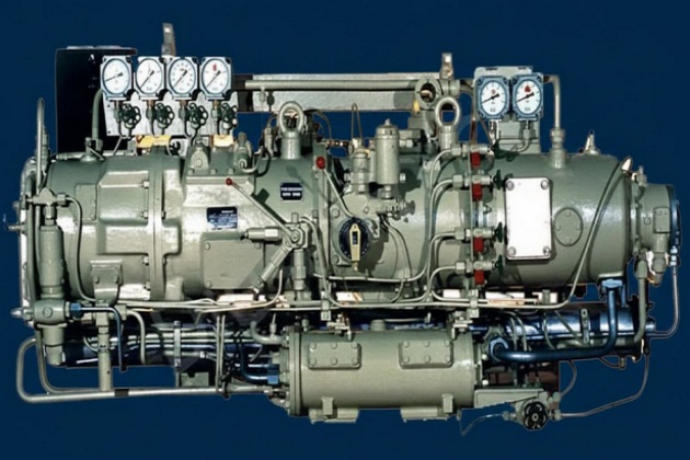
Compressors Configurations
Because gas pipeline projects demand high amounts of capital expenditure and therefore are involved with investments risks, the project sponsor will try to maximize the capacity usage and minimize investment so as to have a competitive transportation rate to offer to the market. At the same time it will avoid the pipeline to operate with spare capacity. The decision on the compressors arrangement whether series or parallel is mostly based on economics and on simulation of failure analysis.
Reduction and Metering Stations
Each reduction and metering station branches off the pipeline and is used to reduce pressure and meter the gas to the various users. For the reduction and metering stations the main equipment includes filters, heaters, pressure reduction and regulators, and flow metering skids. In addition, each station is generally equipped with drains collection and disposal, instrument Inert Gas Systems – Design, Operation, Control Mechanismsgas system, and Shore Natural Gas Storage Tanksstorage tanks.
Filters. Natural gas filter units are installed at each station to remove any entrained liquids and solids from the gas stream. The filters may comprise cyclonic elements to centrifuge particles and liquids to the sides of the enclosing pressure vessel. These particles and liquids will then drop down for collection in a sump, which can be drained periodically.
Source: Pixabay.com
Heaters. Natural gas heaters are installed to avoid the formation of hydrates, liquid hydrocarbons, and water as a result of pressure reduction. The gas heater is designed to raise the temperature of the gas such that after pressure reduction, the temperature of the gas will be above the dew point temperature at operating conditions and maximum flow. The heater is a water bath natural circulation type maintained at a temperature between 158 and 176 °F. Where gas cost is high, an alternative is to use high-efficiency or condensing furnaces for the purpose of preheating the gas rather than the water bath heater.
Pressure Reduction and Regulation System. The pressure reduction system controls the supply pressure to the gas users at a regulated value. Each system consists of at least two trains of pressure reduction, one operating and the other standby. Each train will normally comprise two valves in series, one being the “active valve” and the other the “monitor valve“. Each valve will be equipped with a controller to operate the valve to maintain the preset discharge pressure.
Metering System. The flow rate of the gas has to be measured at a number of locations for the purpose of monitoring the performance of the pipeline system and more particularly at places where “custody transfer” takes place, which is where gas is received from the supply source and gas is sold to the customer for distribution. Depending on the purpose for metering, whether for performance monitoring or for sales, the measuring techniques used may vary according to the accuracy demanded. Typically, a custody transfer metering station will comprise one or two runs of pipe with a calibrated metering orifice in each run.
Design Considerations of Sales Gas Pipelines
The typical design of a gas transmission pipeline involves a compromise among the pipe diameter, compressor station spacing, fuel usage, and maximum operating pressure. Each of these variables influences the overall construction and operating cost to some degree, hence an optimized design improves the economics of the construction and operation of the system and the competitiveness of the project.
Line Sizing Criteria
The pipe size generally is based on the acceptable pressure drop, compression ratio, and allowable gas velocities. Acceptable pressure drop in gas transmission pipelines must be one that minimizes the size of the required facilities and operating expenses such as the pipe itself, the installed compression power, the size and number of compressors, and fuel consumption. In fact, a large pressure drop between stations will result in a large compression ratio and might introduce poor compressor station performance. Experience has shown that the most cost-effective pipeline should have a pressure drop in the range between 3,50 and 5,83 psi/mile. However, for those pipelines (short ones) in which pressure drop is of secondary importance, the pipe could be sized based on fluid velocity only. The flow velocity must be kept below maximum allowable velocity in order to prevent pipe erosion, noise, or vibration problems, especially for gases that may have a velocity exceeding 70 ft/sec. In systems with CO2 fractions of as low as 1 to 2 %, field experiences indicate that the flow velocity should be limited to less than 50 ft/sec because it is difficult to inhibit CO2 corrosion at higher gas velocities.
It will be interesting: The Role of LNG Bunkering Infrastructure
In most pipelines, the recommended value for the gas velocity in the transmission pipelines is normally 40 to 50 % of the erosional velocity. As a rule of thumb, pipe erosion begins to occur when the velocity of flow exceeds the value given by Equation 22:
where:
- Ve – is erosional flow velocity, ft/sec;
- ρG – is density of the gas, lb/ft3;
- and C – is empirical constant.
In most cases, C is taken to be 100. However, API RP 14E suggested a value of C = 100 for a continuous service and 125 for a noncontinuous service. In addition, it suggests that values of C from 150 to 200 may be used for continuous, noncorrosive or corrosion controlled services if no solid particles are present.
After selecting the appropriate inside diameter for a pipe, it is necessary to determine the pipe outside diameter (wall thickness), which would result in the minimum possible fabrication cost while maintaining pipeline integrity.
Example 2
Given the following data for a pipe segment of a gas transmission line, calculate the erosional velocity, neglecting the gas viscosity effect.
- Qsc = 25,7 MMscfd
- Ta = 90 °F
- γG = 0,7
- Za = 0,925
- P1 = 425 psia
- L = 8 280 ft
- D = 12 inch
- E = 1,0
Solution
1 The outlet gas pressure is computed using the Panhandle “A” equation:
2 Calculate the average pressure and gas density:
3 The erosional velocity is computed using API RP 14E equation [Equation 22]. Continuous service (C = 100) is assumed.
4 Check the gas velocities through the line to ensure that excessive erosion will not occur.
The actual gas flow rate is calculated as:
Therefore, the gas velocity is:
The gas velocity is below the erosional velocity, so erosion should not be expected. However, it is high enough to prevent solids from settling.
Compressor Station Spacing
In long-distance gas transmission systems with a number of operating compressors, there is a definite need to optimize the spacing between compressor stations. Compressor station spacing is fundamentally a matter of balancing capital and operating costs at conditions, which represent the planned operating conditions of the transmission system. The process can become somewhat involved and lengthy, particularly as the selection of spacing needs to be designed in such a way to address a capacity ramp-up scenario that will cover not only the initial condition, but also the future years associated with the economics of the pipeline. In case of unexpected growth opportunities we can also rely on loop lines, which may be a better additional choice to increase capacity even more.
For a given pipe diameter, the distance between compressor stations may be computed from the gas flow equation, assuming a value of pipeline operating pressure (station discharge pressure) and a next compressor station suction pressure limited to the maximum compression ratio adopted for the project. Ideally, the pipeline should operate as close to maximum allowable operating pressure (MAOP) as possible, as high density in the line of the flowing gas gives best efficiency. This would point to the selection of close compressor station spacing, but this approach would not be the best economical decision. A decision based on the pipeline economics is the recommended one.
Source: AI generated imageSales Gas Transmission
Based on the required gas flow, an initial diameter is assumed that results in a reasonable compression ratio (usually around 1,3-1,4 for transmission lines) and gas velocity, and the compressor station spacing is established by setting the maximum discharge pressure at the MAOP.
Other diameters are tested, and compressor station spacing calculations are performed again. The optimum diameter is determined based on minimizing capital cost and operating cost, resulting in a chart (the so-called J curves because of their shape) that will plot transportation ratio in US$/MMBTU against transportation capacity based on predefined economic assumptions and risks. Such assumptions include the design life of the facility, the required rate of return on capital employed, and the discount factor used to express the annual operating expenses incurred over time to a present value. The total cost is then plotted against compressor-discharge pressure, and a point of discharge pressure corresponding to the minimum total cost is picked as the best operating pressure.
Note that a good approach is to design for maximum capacity and define the required number of compressor stations and their spacing and after that going down on capacity on each operating year and take stations off as required. This approach will allow a better design and helps defining equipment that would equal. This also allows defining the installation schedule for the compressor stations and compressor units as well.
Capital expenditure (CAPEX) includes costs such as pipe, valves, fittings, compressors, turbines (or electric motors), control and construction, and assembly costs. Operating expenditure (OPEX) includes all maintenance and supervision and fuel or energy cost. CAPEX can be derived from past experience and databases. OPEX has to be estimated based on the specific project and past experience. The most significant part of operating costs is fuel or energy and equipment overhaul. Fuel cost is directly related to compressor horsepower. In order to illustrate how compressor station spacing influences the economics of pipeline operation, a simple model can be set up. This hypothetical pipeline model is based on a system 1 000 miles long, operating at a maximum pressure of 1 000 psig and flowing 1 000 MMscfd. Assuming a uniform pressure loss per unit length of the pipe and station spacing, the inlet pressure at the first station downstream can be calculated and the horsepower needed to bring the pressure up to the discharge pressure setpoint. The process is repeated and the total power needed is the sum of all the stations.
Figure 2 shows the manner in which total power required increases with spacing of stations.
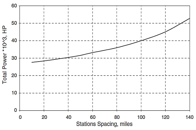
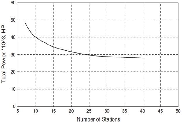
Figure 3 based on the same data shows horsepower in relation to number of stations. We need to keep in mind that even if we have an increase in required power for a pipeline with less compressor stations, the overall cost tends to be lower than many compressor stations with lower horsepower requirements. The installed cost per horsepower will be lower for larger compressor units, and thermodynamic performance will be much better pointing to the direction of having fewer compressor stations with larger compressor units. This explains why an economic evaluation has to be done for each project configuration, taking into consideration all related information in terms of CAPEX and OPEX.
Because fuel use is related to horsepower, a minimum operating cost is associated with close compressor station spacing, which is logical, as maximum transmission efficiency is obtained at the highest mean line pressure, although the pipeline will have a larger diameter, requiring higher CAPEX. However, the optimum is influenced by two factors, the first that small turbine compressor units are less efficient than large ones (have a higher specific fuel consumption), although this effect is small and almost negligible at unit powers above 20 000 horsepower. A much greater impact though lies in the cost of the stations, and this capital cost declines as the number of stations is reduced (not linear as large stations are proportionately more costly than small ones). This tends to move the optimum spacing away from the minimum distance shown in Figure 2.
Every project has to be considered individually because of specific factors and the relationship between CAPEX and OPEX that will differ, but the general conclusion that close spacing results in greater transmission efficiency although may not be the best economic selection.
Experience shows that large units (compressor stations) are more efficient than smaller ones, as larger centrifugal compressors and gas turbines have better efficiency. However, the impact of unit outage or failure must be simulated under a transient analysis so that we can define the remaining capacity and therefore establish a maintenance criterion in terms of having standby units or spare equipment to allow quick replacing without affecting the contractual obligation in terms of transportation capacity.
When the preferred solution is found, it must be tested for robustness not only over the range of throughput anticipated, but also for all credible upset conditions. Having developed the optimum solution the result should then be applied to the practical case with elevation changes and other local factors, including the availability of sites, all of which may result in adjustments and minor changes.
Compression Power
The next step in the design of a pipeline system is to calculate the maximum power required at the stations and set the design point(s). Typically, a new pipeline system will grow from a low flow condition to the maximum over a period of several years, and the decisions on compressors and drivers have to take these changing conditions into account. Growth of flow can be accommodated in several ways. Initially, compressors may only be installed at alternate stations and the intermediate stations built as the growth of flow dictates. Another option is to install one unit at each station location and then add units at the stations as flow increases.
It will be interesting: LNG Bunkering Risk Assessment Worksheet Templates
On the design phase the capacity ramp up will determine the installation schedule for the compressor station and also the additional units that will be necessary at the stations. Hydraulic simulators in both steady and transient states will help make an accurate design and will guarantee that the project will have good performance along the operating years without any unexpected situation. A preselection of the compressor units can also be performed while at the design phase.
Another important job that can be checked in transient analysis is the pipeline operating points inside the performance maps of the compressors on an early basis so as to allow proper selection of impellers and number of compressor units as the capacity increases yearly. Different compressor manufacturers can be modeled to check performance and fuel usage. Operations close to surge line or operations that would require recycling would also be identified during transient analysis underlying the importance of doing this kind of simulation on the design phase of a pipeline.
When the compressor design point is decided, the power required from the driver can be calculated using Equation (Reciprocating and Centrifugal Compressor Comparison for Natural Gas Compression“Formula for actual gas flow rate under suction conditions”).
Pilpeline Operations
In the industry supply chain, pipeline operations is an integral part of the transportation between exploration and production (E&P) or the “upstream end” precedes it and distribution or the “downstream end” follows it. Pipeline operations evolved from being prescriptive (i. e., defined by mandatory requirements) to its current stance of being performance-based driven by risk management principles.
These trends stemmed from competitive forces that decrease operating costs; they also have been evolved because of the experience gained from several decades of pipeline operations along with the technologies and applications that developed along the way. These evolutions have given pipeline operators the tools they need to survive under these conditions. The pipeline facilities are mature to the point that many of them have exceeded their originally intended design life of approximately 25 years at the time of conception. Today, most of these facilities continue to operate, partly for economic reasons as they are too costly to replace and also partly because these facilities still remain worthy of continued use (i. e., they are still deemed to be safe). Recognizing this, operating companies continue to extract value from these facilities, but under tremendous scrutiny and heightened awareness of their existence and vulnerabilities.
Source: Pixabay.com
Current pipeline operation activities have taken on a new dimension of performance. While the basic activities continue, such as mechanical operations and maintenance of the facilities, including line pipe, valves, and valve actuators, corrosion prevention and control, and pipeline monitoring as well as the focus on safety, the optimization of resources is being considered while still achieving safety, reliability, and efficiency. These challenges become more daunting given the fact that these pipeline systems have expanded and merged, often acquiring systems built by others under different design, construction, and operating philosophies. Further, staff reorganization and attrition saw much of the corporate knowledge and information misfiled or discarded. Some companies remained as free-standing, whereas many became a part of a larger corporate entity.
To overcome these developments, pipeline operators now strive for standardization in their procedures and compare their performance to industry benchmarks to gauge their performance and identify areas for improvement.
Certain time-dependent defects such as corrosion and environmental concerns started to manifest themselves in unplanned incidents. Development of other infrastructure at or near pipeline right-of-way saw an increase in third-party incidents and close calls. Pipeline regulators too evolved over these times and increased their vigil over the industry but allowed them to formulate their own facility management programs. Industry sponsored research programs to better understand the consequence effects of pipeline incidents for risk evaluation.
Consequently, pipeline operation has been transformed toward the following areas of focus.
a Making effective choices among risk-reduction measures.
b Supporting specific operating and maintenance practices for pipeline subject to integrity threats.
c Assigning priorities among inspection, monitoring, detection, and maintenance activities.
d Supporting decisions associated with modifications to pipelines, such as rehabilitation or changes in service.
These focus points require that pipeline operations activities include the following elements.
1 Baseline assessment and hazard identification.
2 Integrity assessment by:
a In-line inspection;
b Hydrostatic testing;
c Direct assessment;
d Defect management and fitness for service;
e Information management and data integration;
f Risk management.
3 Integrity management programs.
4 Operator qualification and training.
5 Operating procedures, including handling abnormal operating conditions.
6 Change management.
7 Operating excellence.
These elements constitute a broad makeup of pipeline operations. Not only must operators be aware of them but they must also be well versed in their application, improve them continuously, and incorporate them into a comprehensive and systematic integrity management plan.
Combined, these elements form the basis for directing a prevention, detection, and mitigation strategy for their system.
Read also: Basic Knowledge of Hazard Controls
Pipeline operations will be the longest phase of the life cycle of a pipeline when cost management becomes a high priority. This priority will see pipeline operators performing many scenarios of life extension of the existing assets for enhancing value to its stakeholders.

- API RP 14E, “Design and Installation of Offshore Production Platform Piping Systems”, 4th Ed. Production Department, API, Dallas, TX (April 1984).
- Asante, B., “Two-Phase Flow: Accounting for the Presence of Liquids in Gas Pipeline Simulation”. Paper presented at 34th PSIG Annual Meeting, Portland, Oregon (October 23-25, 2002).
- Aziz, K., and Ouyang, L. B., Simplified equation predicts gas flow rate, pressure drop. Oil Gas J. 93(19), 70-71 (1995).
- Beggs, H. D., “Gas Production Operations”. OGCI Publications, Oil and Gas Consultants International, Inc., Tulsa, OK (1984).
- Brill, J. P., and Beggs, H. D., “Two-Phase Flow in Pipes”, 6th Ed. Tulsa University Press, Tulsa, OK (1991).
- Buthod, A. P., Castillo, G., and Thompson, R. E., How to use computers to calculated heat pressure in buried pipelines. Oil and Gas J. 69, 57-59 (1971).
- Campbell, J. M., Hubbard, R. A., and Maddox R. N., “Gas Conditioning and Processing”, 3rd Ed. Campbell Petroleum Series, Norman, OK (1992).
- Carroll, J. J., “Natural Gas Hydrates: A Guide for Engineers”. Gulf Professional Publishing, Amsterdam, The Netherlands (2003).
- Cleveland, T., and Mokhatab, S., Practical design of compressor stations in natural gas transmission lines. Hydrocarb. Eng. 10(12), 41-46 (2005).
- Colebrook, C. F., “Turbulent Flow in Pipes with Particular Reference to the Transition Region between the Smooth and Rough Pipe Laws”. J. Inst. Civil Engineers, 11, 133-156, London (1939).
- Constantinides, A., and Mostoufi, N., “Numerical Methods for Chemical Engineers with MATLAB Applications”. Prentice Hall, New Jersey (1999).
- Edalat, M., and Mansoori, G. A., Buried gas transmission pipelines: Temperature profile prediction through the corresponding states principle. Energy Sources 10, 247-252 (1988).
- Garland, W. J., Butler, M., and Saunders, F., “Single-Phase Friction Factors for MNR Thermalhydraulic Modeling”. Technical Report, McMaster University, Ontario, Canada (Feb. 23, 1999).
- Goulter, D., and Bardon, M., Revised equation improves flowing gas temperature prediction. Oil Gas J. 77, 107-108 (1979).
- Hughes, T., “Optimum Pressure Drop Project”. Facilities Planning Department Internal Reports, Nova Gas Transmission Limited, Calgary, Alberta, Canada (1993).
- Huntington, R. L., “Natural Gas and Natural Gasoline”. McGraw-Hill, New York (1950).
- Ikoku, C. U., “Natural Gas Production Engineering”. Wiley, New York (1984).
- Jain, A. K. “An Accurate Explicit Equation for Friction Factor”. J. Hydraulics Div. ASCE 102, HY5 (May 1976).
- Kennedy, J. L., “Oil and Gas Pipeline Fundamentals”, 2nd Ed. Pennwell, Tulsa, OK (1993).
- Kumar, S., “Gas Production Engineering”. Gulf Professional Publishing, Houston, TX (1987).
- Lervik, J. K., et al., “Direct Electrical Heating of Pipelines as a Method of Preventing Hydrates and Wax Plugs”. Proceeding of the International Offshore Polar Engineering Conference, 39-45, Montreal, Canada (May 24-29, 1998).
- Maddox, R. N., and Erbar, J. H., “Gas Conditioning and Processing: Advanced Techniques and Applications”. Campbell Petroleum Series, Norman, OK (1982).
- Mohitpour, M., Golshan, H., and Murray, A., “Pipeline Design and Construction: A Practical Approach”. ASME Press, American Society of Mechanical Engineers, New York (2002).
- Mokhatab, S., and Santos, S., Fundamental principles of the pipeline integrity: A critical review. J. Pipeline Integr. 4(4), 227-232 (2005).
- Moody, L. F., Friction factors for pipe flow. Trans. ASME 66, 671-684 (1944).
- Neher, J. H., The temperature rise of buried cables and pipes. Trans. AIEE 68(1), 9 (1949).
- Norsok Standard, “Common Requirements: Process Design”. P-CR-001, Rev. 2, Norwegian Petroleum Industry, Norway (Sept., 1996).
- Nikuradse, J., “Stromungsgesetze in Rauhen Rohren”. Forschungsheft, Vol. B, VDI Verlag, Berlin (July/Aug., 1933).
- Ouyang, L.-B., and Aziz, K., Steady state gas flow in pipes. J. Petr. Sci. Eng. 14, 137-158 (1996).
- Santos, S. P., “Transient Analysis: A Must in Gas Pipeline Design”. Paper presented at 29th PSIG Annual Meeting, Arizona (Oct. 15-17, 1997).
- Santos, S. P., “Series or Parallel: Tailor Made Design or a General Rule for a Compressor Station Arrangement?” Paper presented at 32nd PSIG Annual Meeting, Savannah, GA (Oct. 28-30, 2000).
- Santos, S. P., and Saliby, E., “Compression Service Contract: When Is It Worth?” Paper presented at 35th PSIG Annual Meeting, Berne, Switzerland (Oct. 15-17, 2003).
- Schilichting, H., “Boundary Layer Theory”, 7th Ed. McGraw-Hill, New York (1979).
- Schroeder, D. W., “A Tutorial on Pipe Flow Equations”. Paper presented at 33rd PSIG Annual Meeting, Salt Lake City, UT (Oct. 17-19, 2001).
- Serghides, C. K., Estimate friction factors accurately. Chem. Eng. 63-64 (1984).
- Smith, R. V., “Practical Natural Gas Engineering”, 2nd Ed. Pennwell, Tulsa, OK (1990).
- Streeter, V. L., and Wylie, E. B., Natural gas pipeline transient. SPE J. 10, 357-364 (1970).
- Streeter, V. L., and Wylie, E. B., “Fluid Mechanics”. McGraw-Hill, New York, (1979).
- Towler, B. F., and Pope, T. L., New equation for friction factor approximation developed. Oil Gas J. 92(14), 55-58 (1994).
- Towler, B. F., and Mokhatab, S., New method developed for siting line heaters on gas pipelines. Oil Gas J. 102(11), 56-59 (2004).
- Uhl, A. E., NB-13 Committee, “Steady Flow in Gas Pipelines”. Institute of Gas Technology, Report No. 10, American Gas Association, New York (1965).
- Weymouth, T. R., “Problems in Natural Gas Engineering”. Trans. ASME, Reference No. 1349, 34 (1912).
- Zagarola, M. V., “Mean Flow Scaling of Turbulent Pipe Flow”. Ph.D. thesis, Princeton University, Princeton (1996).